Tag Archives: handle

If You Think You Are Buying Into Oil, Think Again!

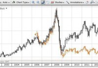
Summary Difficulty in finding a spot oil exposure in the market. USO ETF does not mirror oil price movements perfectly. Long dated oil futures might provide better exposure. There is a lot of hype now looking at oil given the large volatile swings in oil price and its overall drastic decline since about a year ago. For savvy investors, this article would probably not be very relevant because you might already know this. Retail investors who read about oil prices in the news and are very new to this should however, take a closer look. The average investor would probably think of going long or short oil via exchange traded funds, namely the United States Oil Fund or USO. Some information on USO ( website ) As of Jan. 13, 2015 Market Capitalization : 1,688 million Assets Under Management: 1,667 million Management Fee: 0.45% Total Expense Ratio: 0.76% (from 9.30.2014 fund update ) According to the USO website, USO is “designed to track the daily price movements of the West Texas Intermediate (“WTI”) light, sweet crude oil”. For retail investors, this is generally a liquid counter with an average of 16.7 million shares traded daily in the past 3 months. Notably, trading volumes seems to have picked up recently perhaps because of the coverage of oil prices in the news lately. As of Jan 13, the daily volume was 33 million shares traded. Caution is Advised If an investor wants to get exposure to Spot Oil prices without renting a vessel to physically store oil, the investor may have a wrong impression that a good way would be to buy or sell the USO ETF units. Here’s why this is quite ill advised. (click to enlarge) Plotting a chart of the USO ETF with the continuous CLc1 NYMEX prices shows a very obvious trend. In 2009, WTI prices rose from $40 to $80 in a year’s time. During the same period, USO ran up from $29 to $39. A very striking difference in the return profile for an investor who wishes to invest in spot oil prices but ends up buying something different. As prices collapsed in the middle of 2014, from about $100 to right now hitting $45, the USO declined from $37 to about $18. This is also slightly less than the CLc1 movement. For those interested in some numbers, I have extracted out the month-end closing prices of both the USO and the CLc1 in the table below. Month USO CLC1 (spot) USO +/- % CLC1 +/- % Jan-09 29.22 41.75 Feb-09 27.03 44.12 -7.49% 5.68% Mar-09 29.05 48.85 7.47% 10.72% Apr-09 28.63 50.88 -1.45% 4.16% May-09 36.41 66.95 27.17% 31.58% Jun-09 37.93 70.6 4.17% 5.45% Jul-09 36.81 69.5 -2.95% -1.56% Aug-09 36.05 69.57 -2.06% 0.10% Sep-09 36.19 70.4 0.39% 1.19% Oct-09 39.31 76.99 8.62% 9.36% Nov-09 39.16 76.42 -0.38% -0.74% Dec-09 39.28 79.62 0.31% 4.19% Jan-10 35.64 72.64 -9.27% -8.77% Feb-10 38.82 79.61 8.92% 9.60% Mar-10 40.3 83.38 3.81% 4.74% Apr-10 41.33 86.22 2.56% 3.41% May-10 34.05 74.09 -17.61% -14.07% Jun-10 33.96 75.37 -0.26% 1.73% Jul-10 35.34 78.99 4.06% 4.80% Aug-10 31.91 71.68 -9.71% -9.25% Sep-10 34.84 79.81 9.18% 11.34% Oct-10 35.14 81.92 0.86% 2.64% Nov-10 36.04 83.59 2.56% 2.04% Dec-10 39 91.4 8.21% 9.34% Jan-11 38.61 92.22 -1.00% 0.90% Feb-11 39.19 96.87 1.50% 5.04% Mar-11 42.58 106.79 8.65% 10.24% Apr-11 45.15 113.42 6.04% 6.21% May-11 40.5 102.59 -10.30% -9.55% Jun-11 37.26 95.12 -8.00% -7.28% Jul-11 37.43 95.86 0.46% 0.78% Aug-11 34.51 88.72 -7.80% -7.45% Sep-11 30.5 78.75 -11.62% -11.24% Oct-11 35.74 92.58 17.18% 17.56% Nov-11 38.78 100.5 8.51% 8.55% Dec-11 38.11 99.06 -1.73% -1.43% Jan-12 37.82 98.28 -0.76% -0.79% Feb-12 40.92 106.91 8.20% 8.78% Mar-12 39.23 102.93 -4.13% -3.72% Apr-12 39.68 104.89 1.15% 1.90% May-12 32.61 86.5 -17.82% -17.53% Jun-12 31.82 84.84 -2.42% -1.92% Jul-12 32.68 87.96 2.70% 3.68% Aug-12 35.89 96.56 9.82% 9.78% Sep-12 34.13 92.1 -4.90% -4.62% Oct-12 31.78 86.01 -6.89% -6.61% Nov-12 32.56 88.94 2.45% 3.41% Dec-12 33.36 91.79 2.46% 3.20% Jan-13 35.28 97.41 5.76% 6.12% Feb-13 33.06 91.83 -6.29% -5.73% Mar-13 34.76 97.28 5.14% 5.93% Apr-13 33.16 93.32 -4.60% -4.07% May-13 32.61 91.61 -1.66% -1.83% Jun-13 34.15 96.49 4.72% 5.33% Jul-13 37.36 105.32 9.40% 9.15% Aug-13 38.48 107.76 3.00% 2.32% Sep-13 36.85 102.29 -4.24% -5.08% Oct-13 34.69 96.24 -5.86% -5.91% Nov-13 33.46 92.78 -3.55% -3.60% Dec-13 35.32 98.7 5.56% 6.38% Jan-14 34.8 97.46 -1.47% -1.26% Feb-14 36.74 102.76 5.57% 5.44% Mar-14 36.59 101.56 -0.41% -1.17% Apr-14 36.32 99.68 -0.74% -1.85% May-14 37.68 102.93 3.74% 3.26% Jun-14 38.88 105.51 3.18% 2.51% Jul-14 36.31 97.65 -6.61% -7.45% Aug-14 35.76 95.84 -1.51% -1.85% Sep-14 34.43 91.32 -3.72% -4.72% Oct-14 30.63 80.7 -11.04% -11.63% Nov-14 25.58 65.99 -16.49% -18.23% Dec-14 20.36 53.71 -20.41% -18.61% Slight percentage variations in price movements can mean quite a lot to investors. Hence, it is better to understand why this occurs before making a decision to invest. Oil futures are currently in a contango, which basically means oil prices in the future, are worth more than the current price. This usually reflects some cost of handling and storage and cost of carry. (click to enlarge) Looking at the difference between a Dec 2015 futures price of $53.32 versus the front month futures price of $45.99, it may be easy for anyone to simplistically try to mirror a hedge strategy by trying to buy the USO and selling the Dec 2015 futures. The problem lies with how the USO is priced. Here is a snapshot of what the USO holds in its Net Asset Value disclosed: (click to enlarge) (click to enlarge) As shown above, as time progresses, the fund rolls over its holdings from the current front month futures (e.g. Feb 15 futures) into the next month (Mar 15 futures). In the process of rolling over its holdings, it sells the Feb 15 futures and buys the Mar 15 futures, hence incurring the differential cost or spread between the Feb and Mar products. In the USO prospectus page 18, this phenomenon is explained and illustrated in the example quoted below. “If the futures market is in contango, the investor would be buying a next month contract for a higher price than the current near month contract. Using again the $50 per barrel price above to represent the front month price, the price of the next month contract could be $51 per barrel, that is, 2% more expensive than the front month contract. Hypothetically, and assuming no other changes to either prevailing crude oil prices or the price relationship between the spot price, the near month contract and the next month contract (and ignoring the impact of commission costs and the income earned on cash and/or cash equivalents), the value of the next month contract would fall as it approaches expiration and becomes the new near month contract with a price of $50. In this example, it would mean that the value of an investment in the second month would tend to rise slower than the spot price of crude oil, or fall faster. As a result, it would be possible in this hypothetical example for the spot price of crude oil to have risen 10% after some period of time, while the value of the investment in the second month futures contract will have risen only 8%, assuming contango is large enough or enough time has elapsed. Similarly, the spot price of crude oil could have fallen 10% while the value of an investment in the second month futures contract could have fallen 12%. Over time, if contango remained constant, the difference would continue to increase.” Conclusion I hope I have driven the point across on the USO ETF, that it is a means to get exposure to oil price movements, but it is nowhere near a perfectly correlated product.

Protect Profits By Implementing A Risk Reduction Strategy

Improve Returns by Staying Out of Trouble. The Importance of Implementing a Circuit Breaker. Is It Working? Back-Testing Issues Explored. Portfolio return and risk are bound together, but there is a way to minimize losses most investors endure in long bear markets of the type experienced in 2008 and early 2009. How does it work? The sample portfolio described below is made up of ten randomly selected dividend aristocrat stocks plus the Vanguard Total Stock Market ETF (NYSEARCA: VTI ), and two treasury ETFs, the iShares 20+ Year Treasury Bond ETF ( TLT) and the iShares 1-3 Year Treasury Bond ETF ( SHY). VTI and TLT are included as references for equity and bond performance levels. SHY is critical as it is the “circuit breaker” ETF. In other words, reduce portfolio draw-down by staying away from securities that under-perform SHY. Investors will populate the ranking spreadsheet with their own holdings. The sample portfolio holds stocks and ETFs for demonstration purposes only. SHY is the exception as it serves as the ranking cutoff ETF. In the sample portfolio below, an investor holding these securities would sell off Johnson & Johnson ( JNJ), AT&T (NYSE: T ), Coca-Cola (NYSE: KO ), and Chevron (NYSE: CVX ) as these four stocks are ranked below SHY based on three metrics (these three metrics are defined in greater detail in prior Seeking Alpha articles ): Performance over the past 91 calendar days. Performance over the past 182 days. Volatility as measured by a semi-variance calculation. The investing model is as follows. Sell securities that are under-performing SHY based on a performance and volatility ranking model. Purchase the top ranked securities. Depending on how much one wishes to concentrate the portfolio the number of securities will vary. I prefer to work with ETFs so I will rank 10 to 15 Exchange Traded Funds and purchase two to five of them so long as they are ranked above SHY. If no securities are ranked above SHY, then hold the cash in a money market or invest in SHY as it is a low volatile security. (click to enlarge) I’m frequently asked, how well does this model perform when back-tested? Any investment model, when back-tested, is prone to all sorts of uncertainty. Here are a few that quickly come to mind. Stocks and ETFs are purchased throughout the trading day whereas back-tests use closing day prices. Price differences over a multi-year study add significant uncertainty into the final performance results. Many investors use limit orders so it may be days before a limit order is struck and there are times when the order is never placed. The start and end dates of a back-test has a major impact on the end performance results. When using ETFs for back-testing, many do not have years of historical data, thus crippling the results. In the above rankings, how many securities are selected for investment? If two work best in the study how can one be sure it will work out best going forward? Many back-tests “over curve-fit” only to deceive the reader. Is the model an anomaly that will disappear as more investors use it? Staying out of trouble has yet to be fully tested as this model has only been operational for less than one year. Nevertheless, the results are positive when working with ETFs that cover broad indexes such as U.S. REITs, Commodities, Gold, International Bonds, U.S. Bonds, U.S. Equities, International REITs, etc. I am tracking the performance of eleven portfolios, each with a different launch date. Each portfolio is reviewed every 33 days and the reviews are scattered throughout the month. Portfolios are analyzed to see if the performance at the end of each week is trending up or down based on the performance six weeks ago. For nearly every portfolio, those trends are positive. While results are reported each week, only trends over many months will answer the question – is this a valid risk reducing model? A “good” bear market will also help to answer the question.

Industrial ETF: XLI No. 6 Select Sector SPDR In 2014

Summary The Industrial exchange-traded fund finished sixth by return among the nine Select Sector SPDRs in 2014. The ETF was especially strong in the fourth quarter of last year, when it advanced 7.06 percent. However, seasonality analysis indicates the fund could be weak in the first quarter of this year. The Industrial Select Sector SPDR ETF (NYSEARCA: XLI ) in 2014 ranked No. 6 by return among the Select Sector SPDRs that cut the S&P 500 into nine sections. On an adjusted closing daily share-price basis, XLI grew to $56.58 from $51.27, an increase of $5.31, or 10.36 percent. Therefore, it trailed its sibling, the Utilities Select Sector SPDR ETF (NYSEARCA: XLU ), and parent proxy, the SPDR S&P 500 Trust ETF (NYSEARCA: SPY ) by -18.38 and -3.11 percentage points, in that order. (XLI closed at $54.93 Tuesday.) XLI also ranked No. 6 among the sector SPDRs in the fourth quarter, when it behaved better than SPY by 2.16 percentage points and worse than XLU by -6.13 points. And XLI ranked No. 4 among the sector SPDRs in December, when it led SPY by 0.23 percentage point and lagged XLU by -3.59 points. Figure 1: XLI Monthly Change, 2014 Vs. 1999-2013 Mean (click to enlarge) Source: This J.J.’s Risky Business chart is based on analyses of adjusted closing monthly share prices at Yahoo Finance . XLI behaved better in 2014 than it did during its initial 15 full years of existence based on the monthly means calculated by employing data associated with that historical time frame (Figure 1). The same data set shows the average year’s weakest quarter was the third, with a relatively small negative return, and its strongest quarter was the fourth, with an absolutely large positive return. Consistent with this pattern last year, the ETF had a small loss in Q3 and a large gain in Q4. Figure 2: XLI Monthly Change, 2014 Versus 1999-2013 Median (click to enlarge) Source: This J.J.’s Risky Business chart is based on analyses of adjusted closing monthly share prices at Yahoo Finance. XLI performed worse in 2014 than it did during its initial 15 full years of existence based on the monthly medians calculated by using data associated with that historical time frame (Figure 2). The same data set shows the average year’s weakest quarter was the third, with an absolutely large positive return, and its strongest quarter was the fourth, with an absolutely larger positive return. It also shows there is a historical statistical tendency for the ETF to struggle in January. Figure 3: XLI’s Top 10 Holdings and P/E-G Ratios, Jan. 13 (click to enlarge) Note: The XLI holding-weight-by-percentage scale is on the left (green), and the company price/earnings-to-growth ratio scale is on the right (red). Source: This J.J.’s Risky Business chart is based on data at the XLI microsite and FinViz.com (both current as of Jan. 13). The World Bank Group became the latest economic observer to offer evidence of a slowdown in the growth of gross domestic product on this planet in the Global Economic Prospects report it released Tuesday. In its most recent semiannual report, the international financial institution based in Washington estimated GDP grew 2.6 percent in 2014, compared with its forecasts of 2.8 percent last June and 3.2 percent last January: Global growth in 2014 was lower than initially expected, continuing a pattern of disappointing outturns over the past several years. Growth picked up only marginally in 2014, to 2.6 percent, from 2.5 percent in 2013. Beneath these headline numbers, increasingly divergent trends are at work in major economies. While activity in the United States and the United Kingdom has gathered momentum as labor markets heal and monetary policy remains extremely accommodative, the recovery has been sputtering in the euro area and Japan as legacies of the financial crisis linger, intertwined with structural bottlenecks. China, meanwhile, is undergoing a carefully managed slowdown. Disappointing growth in other developing countries in 2014 reflected weak external demand, but also domestic policy tightening, political uncertainties and supply-side constraints. In its GEP report, the World Bank also cut its forecasts of GDP growth in 2015, to 3.0 percent from 3.4 percent, and in 2016, to 3.3 percent from 3.5 percent. The conditions underlying these cuts in the World Bank’s forecasts appear likely to have deleterious effects on the earnings of many of XLI’s constituent companies (i.e., those with major exposures to the global economy). This is especially so given the bias divergence in monetary policy at major central banks around the world and its impact on currency-exchange rates, as discussed in “PowerShares QQQ’s 2014 And Fourth-Quarter Performance And Seasonality.” At this late stage of the economic/market cycle, the valuations of XLI’s top 10 and other holdings seem unlikely to function as tailwinds for the ETF’s price appreciation in the foreseeable future (Figure 3). However, the numbers on the S&P 500 industrial sector reported by S&P Senior Index Analyst Howard Silverblatt Dec. 31 suggest it is not hideously overvalued, with its P/E-G ratio at 1.37: not cheap to the likes of me, not dear to the likes of normal people. Disclaimer: The opinions expressed herein by the author do not constitute an investment recommendation, and they are unsuitable for employment in the making of investment decisions. The opinions expressed herein address only certain aspects of potential investment in any securities and cannot substitute for comprehensive investment analysis. The opinions expressed herein are based on an incomplete set of information, illustrative in nature, and limited in scope. In addition, the opinions expressed herein reflect the author’s best judgment as of the date of publication, and they are subject to change without notice.