Tag Archives: seeking-alpha

Lipper Closed-End Funds Summary: December 2014

By Tom Roseen In December the U.S. market took investors on a wild ride. Toward month-end the Dow Jones Industrial Average and the S&P 500 Index posted their thirty-eighth and fifty-second record closes for the year, respectively. A strong nonfarm payroll report at the beginning of the month pushed up U.S. equity markets, and the Dow flirted with the 18,000 mark for the first time. However, concerns about the health of the global economy the following week fueled one of the largest one-week drops in two and half years and sent the VIX to its highest level since October 17. Investors shrugged off a better-than-expected consumer sentiment report and focused on volatility in oil prices and the possibility of the global economy succumbing to deflation. Despite a Federal Reserve-fueled Santa Claus rally toward month-end, U.S. stocks finished the good year on a down note, with the Dow witnessing a triple-digit loss on the last trading day of the month. Both equity and fixed income CEFs posted negative NAV-based returns (-1.43% and -0.24% on average, respectively) for the first month in three, while market-based returns were also in the red for both equity CEFs (-2.51%) and fixed income CEFs (-0.02%). Treasury yields declined at all maturities ten-years or greater in December, with the twenty-year yield declining the most, 15 bps to 2.47% at month-end. The rising dollar and slowing growth overseas made U.S. Treasuries more attractive to foreign investors. The Treasury yield curve rose in most of the lower-dated maturities, with the three-year rising the most-22 bps to 1.10%-by month-end. The one-month yield witnessed a small decline, dropping 1 bp to 0.03%. For December the dollar once again gained against the euro (+2.69%), the pound (+0.32%), and the yen (+0.88%). Commodities prices were mixed, with near-month gold prices rising 0.73% to close the month at $1,184.10/ounce. Meanwhile, front-month crude oil prices plunged a whopping 19.60% to close the month at $53.27/barrel. That equated to a quarterly decline of 40.41% and a one-year decline of 45.87%. For the month 47% of all CEFs posted NAV-basis returns in the black, with 33% of equity CEFs and 58% of fixed income CEFs chalking up returns in the plus column. The slide in oil prices and concerns over Greece’s inability to elect a favored presidential candidate, rekindling fears of another European crisis, weighed on Lipper’s World Equity CEFs macro-classification (-2.43%), pushing it to the bottom of the equity CEF universe. On the equity side (for the fourth consecutive month) mixed-asset CEFs (-0.73%) mitigated losses better than the other macro-groups, followed by domestic equity CEFs (-1.15%). Once again, the municipal bond CEFs group (+1.13%) was the only fixed income macro-classification posting a return on the plus-side for the month, with all of its classifications experiencing returns in the black. The muni CEFs group was followed by domestic taxable bond CEFs (-1.47%) and world bond CEFs (-4.17%). For December the median discount of all CEFs widened just 19 bps to 9.28%-deeper than the 12-month moving average discount (8.55%). Equity CEFs’ median discount widened 115 bps to 9.46%, while fixed income CEFs’ median discount narrowed 53 bps to 9.13%. To read the complete Month in Closed-End Funds: December 2014 FundMarket Insight Report, which includes the month’s closed-end fund corporate events, please click here .

Maybe You Should Be In 100% Cash

This post has nothing to do with asset prices, valuation, or timing the market as the title may have led you to believe. It has to do with investor psychology and behavior. Over the years I’ve wondered if certain types of people would be happier if they didn’t invest in anything but cash. Not ‘better off’ mind you just happier and still able to meet their financial goals – like a successful happy retirement. Then I said, “I have the data for that analysis.” Let’s take a look at the kind of people I’m talking about. You’ll probably see a bit of yourself in my description. Then let’s see what kind of retirement such a person could reasonably expect and some strategies to make it better. I think we all know the type of person I’m alluding to. Most investors have some of these traits. Constantly worried about any kind of investment. Stocks – they’re always too expensive or so cheap it’s an indication of some forthcoming dire event and thus they must continue to go down. International stocks – same thing, even worse. Bonds – even the mighty U.S. government is going default for sure. Any day now. Gold – sure, we gotta have a lot of that but I need to check the prices three times a day. And anytime prices go down it’s manipulation. Inflation – we’re constantly falling behind in standard of living. At the extreme, always worried about large inflation any day now. Yield – the need to reach for yield and check news every day that may affect the income stream. Price fluctuations of any significant amount are a sign to take action and seek refuge. Logging in to investment accounts way more than necessary and checking account balances. Glued to financial news of any kind. Tweaking investments all the time always looking for the better bet. In general, constant unease about the future and definitely not able to sleep comfortably at night. I may be exaggerating a bit but I know quite a few people, young and old, that would fit a large part of this description. And I think a large part of these people can overcome these behavioral obstacles, especially by adapting an automatic investment process or system like the ones I discuss on this blog. But I also often wonder if some people would be better off just sticking with investing in 100% cash and never taking any investment risk. They would be much happier. Let’s take that as a given and see how much could such a person expect to reasonably withdraw from their cash portfolio in retirement (which also determined what size portfolio such a person would need to retire). Let’s find out. Using the database I use to calculate SWRs (see here for an example), I replaced the U.S. 10 year bond returns with the historical series for the U.S. 3 month T Bill from 1929 to 2014 to represent cash returns. This is a pessimistic return series to use for cash returns but it’s the best series with that much history. Normally, even in environments with very low U.S. T Bill rates an investor can get cash returns out to 1 year that are quite a bit higher. For example, even with today’s low T Bill rates of 0.14% or so you can get a 1 year CD at many banks yielding over 1%. Below are the historical SWRs (Safe Withdrawal Rates) for a few scenarios with a 100% cash portfolio. The historical SWR for a 100% cash portfolio is 2.3% using a normal inflation adjusted spending model. That is quite a lot lower than the 4% from a 60/40 U.S. stock bond portfolio but definitely do-able. And definitely a portfolio that would have allowed for many more restful nights. The rest of the table shows what the SWR would be with some tweaks to the spending model. The FCM (floor-ceiling) model adjusts inflation adjusted spending down during bad return years. The spending adjustment column uses the historical fact that retirees’ spending increases less than inflation, between 1-2% less than inflation in fact. Using these better spending models increases the historical SWR to 3.34%. Doesn’t sound too bad now does it? Not too far off from the old 4% rule. But how realistic are these spending scenarios? In my opinion and in my experience the above spending scenarios are easily achievable. Think about what people did before easily accessible and low cost investment options. Investing was something reserved for the wealthy or least very well to do. It’s only in modern times that investing is so widespread and accessible. How did your parents or grandparents plan and survive retirement? If they were like my grandparents they planned and survived retirement through a combination of saving a lot and not spending a lot. There was never any investment talk. Getting them to trust bank CDs took almost 10 years! Yet they made it and were quite happy along the way. Sure, they could have been ‘better off’ but they wouldn’t have been as happy. Now lets turn to a modern and more tangible example, me and my wife Nina. From our base spending level in 2005, we spent 53% less in 2014. Yes, that involved a massive life change. By choice. You can read out it on Nina’s blog and even watch a little video about it. But it was for the better. Infinitely better for us. Oh, and that is in nominal terms. In real dollars, we spend 70% less (inflation has grown 2005 dollars by 20%) than we did in 2005. OK, that’s cheating a bit. At least in the ability to generalize from a very specific and personal choice. So, lets take our spending change since we started RV’ing in 2010. In 2014 we spent 10% less than we did in 2010. Inflation is up 8% since then. In real dollars that means we spend 18% less than we did in 2010. That’s over 3% a year. Obviously that can’t go on forever. And we’re pretty much at the bottom of the curve so to speak. Any further dramatic changes would require a reduction in quality of life which is not acceptable to us. Going forward our goal is to keep spending flat in nominal terms. Worst case to keep pace with inflation. I think that is pretty achievable. Our example just goes to show that controlling your spending so that it grows less than inflation is certainly achievable and not just data from some impersonal random study. The other aspect of future spending is that most people have some type of retirement or pension income that begins in later years. This is mainly social security. So, in order to get a truly realistic picture of the future we need to forecast cashflows on a yearly basis. Then we can get a true picture of what SWRs would look like from a 100% cash portfolio. Kind of like I talked about in this post . Let’s consider a 65 year old couple just beginning retirement, delaying social security until 70, a median social security income of that covers about 40% of their expenses, and controlling their spending so that it grows at 1% less than inflation. Taking this cash flow model and applying it to the historical returns from a 100% cash portfolio gives us a worst case SWR of 4.13% for the 30 year retirement period starting in 1942. Not so harsh a retirement after all. Even in 100% cash. And definitely many more restful nights than an equity heavy portfolio. In conclusion, sometimes taking an extreme position can be quite thought provoking and insightful. Admittedly, that is what I’ve done here. It was also a bit tongue in cheek. I’ve shown that even with a 100% cash portfolio a reasonable retirement can be had by focusing on the other side of the equation, spending, and using some more realistic retirement assumptions. People have been doing it for a long time. A lot longer than they have been investing in broadly diversified portfolios across world wide asset classes and markets. And maybe this thought experiment allows us to worry a bit less about our investments and have some more restful nights for just having thought through these alternative scenarios.

Using Adaptive Asset Allocation To Limit Market Risk And Increase Return

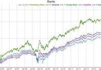
Summary Adaptive asset allocation enables an investor to capture higher returns and reduce risk compared to “buy and hold” and “fixed asset allocation”. Adaptive asset allocation can adjust the portfolio to compensate for varying market conditions. A backtest from Nov 2005 to Jan 2015 shows one allocation strategy resulting in more than double the returns and much less risk compared to a buy and hold strategy. Adaptive asset allocation is often cited as an attractive alternative to fixed or standard asset allocation so popularly used. Standard asset allocation or fixed asset allocation is the idea of allocating 10% of your portfolio to this and 25% to that and another 7% to this asset class and keeping that percentage fixed regardless of market circumstances. Adaptive asset allocation is quite different in how it decides how much is allocated to each asset in a portfolio, instead of using fixed numbers set by an individual or corporation at one time during one market cycle and sticking with it through thick and thin, adaptive asset allocation adjusts or adapts the portfolio weightings on a regular basis based on maximizing or minimizing a certain performance metric such as volatility or variance or even the Sharpe ratio. Market cycles as well as bear markets can be ruinous at worst and challenging at best for most fixed asset allocation models. If you recall 2008, the S&P 500 lost around 55% of it’s value, but Gold didn’t miss a beat until it has lost 1/3 of it’s value from 2011-2013. Bonds surged while the stock market crashed in 2008, but many bonds faltered for much of 2013 while the stock market soared. Certainly you can see why diversifying a portfolio is of great value, but it begs the question “Why did we have to hold on to the stock funds we were invested in?”. The first reason we could cite is a very valid one, and it is because we needed to hold onto it so we could benefit from it in the good years like 2013. The next question you may ask is “Why couldn’t we reduce the amount of money we have in the stock market when it is falling or the bond market when it was falling and why have I been holding so much Gold the last few years?”. This is where a fixed allocation system simply says we set a fixed amount and we stick to it regardless of circumstances, but lets take a look at how adaptive asset allocation answers this question. Enter Adaptive Asset Allocation Adaptive Asset Allocation sets the weight of each asset in your portfolio not by a fixed percentage but as a result of optimizing different performance metrics. For example, we could optimize a portfolio’s weightings to minimize volatility or minimize variance or maximize the risk adjusted return (Sharpe Ratio). Each of these optimization criterion can be used to decide how much of each asset in your portfolio instead of using a fixed percentage. As you can see, adaptive asset allocation answers the questions posed above, namely how can we reduce the allocation in a certain asset when it is doing poorly. We are now going to reduce our assets in an asset that is volatile or has a high variance or a low risk adjust return (Sharpe Ratio), and increase our assets in funds that have low volatility or low variance or a high risk adjusted return. Our Test Now that we have established the rationale for why we might want to use adaptive asset allocation let’s test a sample portfolio to see if Adaptive Asset Allocation can improve returns and reduce drawdown. For this portfolio I am going to use Exchange Trade Funds (ETFs) to select US Stocks, International Stocks, Gold, and US Treasury bonds as our portfolio assets. The tickers used are SPY for US Stocks, EFA for International Stocks, GLD for Gold, and TLT for US Treasury bonds. Parameters We are going to try 3 different performance metrics for deciding our weighting, the first is minimizing volatility, the second is minimizing variance, and the third is maximizing the risk adjusted return (Sharpe Ratio). For all calculations we are just going to use the 3 month trailing volatility, variance, and Sharpe ratio as our measurement. We are going to adjust the portfolio on a monthly basis, this may be too often or not often enough, but for an introduction to these type of ideas it is what we will use. Results – Volatility (click to enlarge) Pink Line is Volatility Returns (click to enlarge) Weightings for each symbol over time (EFA=yellow, GLD=blue, SPY=green, TLT=pink) The performance for the minimum volatility weighted portfolio is: 9.42% CAGR 0.98 Sharpe Ratio 9.72% Volatility 22% maximum draw down This compares to the equally weighted version of this portfolio (25% SPY, 25% GLD, 25% EFA, 25% TLT): 8.5% CAGR 0.76 Sharpe Ratio 11.61% Volatility 28.81% maximum draw down And to the S&P 500 alone: 7.64% CAGR 0.47 Sharpe Ratio 19.96% Volatility 55.22% maximum draw down The minimum volatility adaptive asset allocation portfolio successful outperformed the S&P 500, and equally weighted portfolio in all the performance metrics shown above! As you will see in the transition map image above, the volatility adaptive asset allocation did a lot of what we mentioned to reduce risk; during the 2008 stock market crash the % in SPY and EFA dropped considerably, while the bond fund took over a large percentage of the portfolio, and recently the allocation in gold has been dropping to reduce the exposure to the falling gold market. Results – Variance (click to enlarge) Blue Line is Variance Returns (click to enlarge) Weightings for each symbol over time (EFA=yellow, GLD=blue, SPY=green, TLT=pink) The performance for the minimum variance weighted portfolio is: 10.1% CAGR 1.12 Sharpe Ratio 8.95% Volatility 14.84% maximum draw down The minimum variance adaptive asset allocation portfolio again successful outperformed the S&P 500, and equally weighted portfolio in all the performance metrics shown above! The minimum variance adaptive asset allocation did even more than the minimum volatility portfolio to reduce risk and increase returns. During the 2008 stock market crash the % in SPY and EFA dropped to near 0%, while the bond fund took over the majority of the portfolio, the allocation in bonds dropped while stocks recovered, and recently the allocation in gold has been dropping to near 0% to reduce the exposure to the falling gold market. Results – Risk Adjusted Return (Sharpe Ratio) (click to enlarge) Green Line is Sharpe Ratio Returns (click to enlarge) Weightings for each symbol over time (EFA=yellow, GLD=blue, SPY=green, TLT=pink) The performance for the maximum Risk Adjusted Return (Sharpe Ratio) weighted portfolio is: 15.43% CAGR 1.07 Sharpe Ratio 14.4% Volatility 27.27% maximum draw down The maximum Sharpe ratio adaptive asset allocation portfolio again successful outperformed the S&P 500, and equally weighted portfolio in all the performance metrics shown above – especially returns! The maximum Sharpe Ratio adaptive asset allocation did a lot to increase returns and even managed to outperform in the areas of drawdown and volatility over the S&P 500 and equal weight portfolios. Optimizing the Sharpe ratio is definitely aggressive, you will notice how it often completely eliminates assets from the portfolio and even is only in a single asset during certain times. During the 2008 stock market crash the % in SPY and EFA dropped to 0%, while the bond fund took the entire 100% of the portfolio, the allocation in bonds dropped while stocks recovered and there were many times when stocks where 100% of the portfolio, and recently gold has been almost completely absent from the portfolio even though it played a strong role in the portfolio when it was surging upwards earlier in the backtest. One More Thing… One thing that may be problematic is the fact that some of these allocations involve entirely or nearly getting rid of an investment, especially the Sharpe Ratio portfolio. One thing we can do to combat this is what I call “dampen” the weighting algorithms. This involves “dampening” the effects of each weighting algorithm by only allowing the weighting algorithm to go so far. For example you could decide you want to hold no less than 5% of a certain asset, you could then call 0-4% 5% and adjust the other weightings accordingly to effectively “dampen” the effect of the weighting algorithm to make the portfolio more like a fixed allocation strategy. So lets take a quick look at “dampening” the Sharpe Ratio adaptive asset allocation portfolio to see what a little more conservative switching can do: Results – Risk Adjusted Return (Sharpe Ratio) with ~7% Minimum per Asset (click to enlarge) Green Line is Sharpe Ratio with Dampening Applied (click to enlarge) Weightings for each symbol over time (EFA=yellow, GLD=blue, SPY=green, TLT=pink) The performance for the maximum Risk Adjusted Return (Sharpe Ratio) weighted portfolio with dampening is: 13.68% CAGR 1.13 Sharpe Ratio 12.04% Volatility 24.68% maximum draw down So we reduced the full effect of the Sharpe Ratio weighting and we got a portfolio that did not entirely eliminate any symbol, but also wasn’t afraid to aggressively reduce its allocation in assets when they had a bad risk adjusted return value. The results show a smaller CAGR return %, but improvements in the area of Sharpe Ratio, volatility, and maximum drawdown. Conclusion Adaptive asset allocation can be used to re-weight our portfolio to reduce drawdown and increase returns in the ever changing markets as opposed to a more traditional fixed asset allocation. We tested 3 techniques that can be used to weighted a portfolio and noticed how each responded to the changes in the stock markets, bond markets, and gold market. Each strategy was able to outperform a standard buy and hold approach and the stock market, while also delivering better volatility and draw down numbers in the backtests presented above. With ever increasing uncertainty in the direction of the markets and how best to diversify a portfolio adaptive asset allocation may be one answer of how to eliminate guesswork and provide a foundation for adjusting allocations to compensate for the winds and waves of the markets.