Tag Archives: nreum

Unitil (UTL) Q4 2014 Results – Earnings Call Webcast

The following audio is from a conference call that will begin on January 28, 2015 at 14:00 PM ET. The audio will stream live while the call is active, and can be replayed upon its completion. If you would like to view a transcript of this call, please click here. Now that you’ve read this, are you Bullish or Bearish on ? Bullish Bearish Sentiment on ( ) Thanks for sharing your thoughts. Why are you ? Submit & View Results Skip to results » Share this article with a colleague

The ‘Efficiency’ Of The Market Doesn’t Matter To Smart Investors

The huge growth in index funds has caused some investors to debate the merits of the market’s “efficiency” and whether index funds would make the markets less efficient. The basic thinking is that if everyone starts buying index funds then that could create more opportunities for stock pickers who are able to go against the grain and pick the stocks that have been unjustifiably correlated to the actions of the overall index. This whole debate confuses why correlations are rising in the first place. Correlations aren’t rising because index funds are becoming more prevalent. Index funds are becoming more prevalent because the performance of the economy is becoming increasingly correlated. If you look at any sector of the S&P 500, you’ll find rising correlations over the course of the last 50 years. The average 10-year correlation of all the sectors of the S&P 500 is about 83.5%: (10-Year Correlation of various sectors) This isn’t happening because index funds are becoming more popular. It’s happening because US corporations are becoming increasingly interconnected. Public companies are becoming multi-national and multi-industry companies whose performance depends increasingly on the way the macroeconomy works. If we look at the underlying Earnings Per Share of these same industries, we find equally strong correlations in their profit growth over time. Of course, high correlations doesn’t mean there won’t be uncorrelated entities whose prices get irrationally whipsawed by the aggregate market performance. But it does mean that it is becoming increasingly difficult to find entities who aren’t dependent on the performance of the broader economy. Finding truly uncorrelated companies is not as easy today as it might have been back in the early 1900s when the broader economy was much more fragmented. Paul Samuelson always argued that the markets were micro efficient, but not macro efficient. Indeed, the whole concept of market “efficiency” is becoming increasingly irrelevant in a world where entire economies are becoming so highly correlated. But this doesn’t change the importance of understanding the discussion and its impact. At the aggregate level, we have all become “asset pickers.” The distinction between “active” and “passive” investors is largely irrelevant in a world where we all now pick baskets of assets inside the global aggregate. And when one deviates from global cap weighting (roughly the Global Financial Asset Portfolio) you are engaging in a form of asset picking that makes you no different than a stock picker. You are declaring that you can generate a better risk adjusted return than the global aggregate. Indexing has become the new stock picking. Instead of picking 25 stocks in an index, we now pick baskets of index funds inside a global aggregate. The idea of “market efficiency” was never very useful to begin with however because it is constructed around a gigantic political strawman. The EMH is essentially a political construct that argues that discretionary intervention is useless because “the market” is smarter than everyone else. It is a political argument against discretionary intervention that was constructed to create a theory of finance that was consistent with an anti government economic theory (Monetarism primarily). In essence, you can’t “beat the market” because the market is so smart. This is silly though. The market will generate the aggregate market return and your real, real return will be the market return minus the rate of inflation, taxes and fees. Taxes and fees alone will reduce the aggregate return by over 35% (if we assume a 10% aggregate return, 1% fees and 25% tax rate). No one will consistently beat “the market” aside from a few lucky outliers. The math just doesn’t work. And the index we are comparing ourselves to is a completely fictitious benchmark because the average real, real return is lower than the pre-tax and pre-fee benchmark to begin with. But the EMH defenders have misconstrued this entire debate to promote a political position constructed by anti government economists at the Chicago School of Economics. Imagine, for instance, that, for the purpose of record keeping, at the end of each NBA basketball game, the NBA reduced the average score of 100 points by 25%, and then imagine that the coaches reduced the score by another 10%. What the EMH defenders have done is argued that the score of 100 means that the teams are all terrible because they cannot, on average beat this “benchmark.” There will be outlier teams who sometimes score more than 100 points, but on average these “professional” teams will underperform. EMH defenders have used this strawman to argue that “active” investors are all terrible. It’s a completely useless construct that does nothing more than misconstrue the entire premise of the discussion. Of course, none of this means that high fees and overly active trading are good. After all, when one engages in such activities they only increase the size of the friction, which reduces returns in the first place. But the debate about EMH and “active” vs. “passive” has been blurred by a useless discussion about how “efficient” the market is. The reality is that we are all active investors to some degree. All indexers have to pick their asset allocations and the funds they will use. All indexers time their entry/exit points, their rebalancing points, their “tilts,” etc. The smarter indexer tries to capture much of the broad market gain while reducing their tax and fee burden. But that has nothing to do with whether the market has become “efficient” or whether some degree of “active” management is “smart” or “stupid.” Samuelson was right – the market is micro efficient and macro inefficient. And as the market has become increasingly macro oriented the discussion about the “efficiency” of the market has become increasingly useless.

Safe Withdrawal Rates For Retirement Income Portfolios Using Fidelity Select Mutual Funds

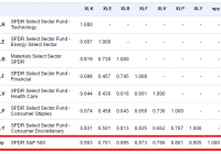
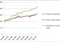
Summary Robust investment portfolios with large withdrawal rates can be constructed with Fidelity select mutual funds. From January 1990 to December 2014, a Fidelity portfolio with fixed allocation allowed a safe 6% annual withdrawal rate and achieved 6.19% annual increase of the capital. Same portfolio with rebalancing at 25% deviation from the target allowed a safe 6% annual withdrawal rate and achieved 7.78% compound annual increase of the capital. Radically better performance is achieved using adaptive asset allocation. Same portfolio allowed a safe 6% annual withdrawal rate and 22.05% annual increase of the capital. The Chicago South Suburban Investment Club has been experimenting with a monthly asset rotation strategy applied to a hypothetic IRA account using five Fidelity mutual funds. On the last trading day of each month, the funds are ranked by the previous 3-month return. All equity is invested in the fund with the highest return, as long as that return is positive. If all the assets had negative returns over the previous 3 months, then all equity is moved into CASH. The five mutual funds considered for investment are the following: Fidelity GNMA (MUTF: FGMNX ) Fidelity Select Multimedia (MUTF: FBMPX ) Fidelity Select Chemicals (MUTF: FSCHX ) Fidelity Select Electronics (MUTF: FSELX ) Fidelity Select Health Care (MUTF: FSHCX ) This experiment has been ongoing since July 2014. It extends over a period of 5 months. Within this time interval, the system had been invested 4 months in FSPHX, 1 month in FSELX, and current month in FLBIX. The results are showed in the table below. Table 1. Momentum allocation portfolio August 2014 to January 2015 Month AUG SEP OCT NOV DEC JAN ETF FSPHX FSPHX FSPHX FSPHX FSELX FLBIX BUY 206.52 218.7 218.92 228.7 81.43 13.32 SELL 218.7 218.92 228.7 236.08 84.78 RETURN 5.90 0.10 4.47 3.23 4.11 EQUITY 100.00 105.90 106.00 110.74 114.31 119.02 In this article, three different strategies will be considered: (1) Portfolio is initially invested 50% in the bond fund , and 12.5% each in the four equity funds without rebalancing. (2) Portfolio is initially invested 50% in the bond fund , and 12.5% each in the four equity funds but is rebalanced when the allocation to any fund deviates by 25% from its target. (3) Portfolio is at all times invested 100% in only one fund. The switching, if necessary, is done monthly at closing of the last trading day of the month. All money is invested in the fund with the highest return over the previous 3 months. The data for the study were downloaded from Yahoo Finance on the Historical Prices menu for the five tickers, FGMNX, FBMPX, FSCHX, FSELX, FSPHX. We use the monthly price data from January 1990 to December 2014, adjusted for dividend payments. The purpose of this exercise is to develop a robust strategy for income generation in retirement. The paper is made up of two parts. In part I, we examine the performance of portfolios without any income withdrawal. In part II, we examine the performance of portfolios when income is extracted periodically from the account. Part I : Portfolios without withdrawals In table 2 we show the results of the portfolios managed for 25 years, from January 1990 to December 2014. Table 2. Portfolios without withdrawals 1990 – 2014. Strategy Total return% CAGR% Number trades MaxDD% Fixed-no rebalance 1,463 11.62 0 -49.21 Fixed-25% rebalance 1,395 11.43 28 -22.55 Adaptive 18,015 23.35 126 -33.11 The time evolution of the equity in the portfolios is shown in Figure 1. (click to enlarge) Figure 1. Equities of portfolios without withdrawals. Source: This chart is based on EXCEL calculations using the adjusted monthly closing share prices of securities. Notice that the prices are shown in a logarithmic scale. That allows a better differentiation between the curves. It is apparent that the rate of increase of the adaptive portfolio is very stable and is substantially greater than the rate of the fixed allocation portfolios. One can also see that rebalancing of the fixed allocation portfolio makes its rate of increase much more stable than that of the portfolio without rebalancing. Part II: : Portfolios with withdrawals Assume that we have $1,000,000 to invest for income in retirement. In table 2 we show the results of the portfolios managed for 10 years, from January 2005 to December 2014. Money was withdrawn monthly at a 6% annual rate of the initial investment plus a 2% inflation adjustment. Over the 10 years from January 2005 to December 2014, a total of $664,704 was withdrawn. Table 3. Portfolios with 6% annual withdrawal rate 2005 – 2014. Strategy Total return% CAGR% Number trades MaxDD% Fixed-no rebalance 122.63 2.06 0 -28.82 Fixed-25% rebalance 125.76 2.32 5 -30.11 Adaptive 278.92 10.8 56 -15.92 The time evolution of the equity in the portfolios is shown in Figure 2. (click to enlarge) Figure 2. Equities of portfolios with 6% annual withdrawal rates. Source: This chart is based on EXCEL calculations using the adjusted monthly closing share prices of securities. Conclusion The adaptive allocation algorithm performed substantially better than the fixed allocation algorithms. The fixed allocation strategies allow a safe withdrawal rate of 6% at any time horizon between 1990 and 2014, without a substantial decrease of capital. The adaptive allocation algorithm allows a 6% annual withdrawal rate while assuring a substantial increase of capital. In fact, the momentum-based adaptive allocation strategy allows a safe 10% annual rate of withdrawal without any decrease of capital.