Tag Archives: gestaltu

GTAA Is For Real (Part 3): Why VBINX Is The Wrong Benchmark

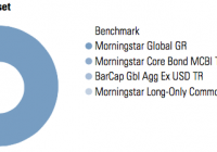
To judge a strategy, it is critically important to identify an appropriate benchmark. For several reasons, comparing tactical strategies to “balanced portfolios” like VBINX is inappropriate. The Global Market Portfolio meets all the criteria for a proper benchmark, making it is the most appropriate baseline for assessing GTAA strategies. At our research blog, we recently posted an article discussing how many noteworthy investment commentators either misunderstand or misconstrue the salient qualities of Tactical Asset Allocation strategies. We encourage you to read the entire piece, but today’s post will be limited to the topic of benchmarking. One of the most common failings of the investment industry is the prevalence of poorly specified benchmarks. This is of critical importance because it’s easy for a knowledgeable but disingenuous professional to manipulate the facts in order to make any point they want. Want a simple way to boost results? Choose an easy benchmark for comparison. Want to dismiss performance? Choose a challenging benchmark. Recall that at root, a well specified benchmark should meet the following criteria: It is passive; It is investible, and; It reflects the investing opportunity set of the manager. While all of these criteria are individually valid, they are unified by a simple and profound benchmarking philosophy: The best benchmark for a tactical manager is the one they would own if everyone were forced to invest all their assets in a single, passive portfolio. Axiomatically, this portfolio would represent the average positions of all market participants, and would hold each asset in a percentage equal to its proportion of total market capitalization. This is not a new concept; U.S. large cap equity managers are typically benchmarked against a market cap weighted index of large-cap U.S. stocks. U.S. Investment Grade bond managers are benchmarked against a market cap weighted index of U.S. listed investment grade bonds. Cap weighted indexes are common and intuitive when they are constructed within a major asset class. But it is not immediately intuitive how to extend the concept to multi-asset universes like those employed by GTAA managers. As a result, GTAA strategy benchmarks often seriously misrepresent the risks and opportunities of the underlying strategies. Investment commentators who dismiss TAA often compare the results of GTAA strategies to a U.S. 60/40 balanced fund like the Vanguard Balanced Index Fund (MUTF: VBINX ). And this benchmark does have one thing going for it, especially if a commentator’s goal is to malign GTAA strategies: it is a very tough benchmark to beat over the past one, three and five years – perhaps the toughest in the world in USD terms. Unfortunately, it’s hard to see how this portfolio represents an appropriate bogey for GTAA strategies over the long-term. For one, this portfolio is insulated from global currency effects, which have been especially pronounced in the past few years with global QE programs in effect. Second, it ignores non-U.S. equity beta; while a focus on U.S. equities at the expense of international stocks has been a lucky bet for the past few years, it ignores the broader scope of GTAA strategies. Also, since the goal of GTAA strategies is to harvest premia from as many liquid global sources as possible, the strategies often incorporate alternative investments, like REIT and commodity ETFs, into their investible universe. These are not represented in a U.S. balanced fund benchmark. Fortunately, some analysts take a more enlightened view. In their quarterly ” ETF Managed Portfolios Landscape Summary ” report, Morningstar proposes a much more globally diversified benchmark. The report’s Global All Asset benchmark, copied below, is composed of 55% global stocks, presumably distributed geographically by market cap; 35% global bonds, split evenly between U.S. and international; and 10% commodities. Source: Morningstar Clearly the folks at Morningstar are trying to be more representative of the GTAA space, and their mix is certainly in the right ballpark. But it is also still rather arbitrary – how did they arrive at their weights? Have they weighted toward historical GTAA holdings? If so, is there any guarantee that historical holdings will be representative of future holdings? These are dynamic strategies after all. Do commodities deserve a 10% strategic weighting or is this informed by recency bias? In addition, the Morningstar benchmark is over 80% weighted to U.S. dollars. Does this represent a neutral currency policy? We stated above that it isn’t immediately obvious how to extend the market cap weighted benchmarks applied to traditional single-asset portfolios, such as equity or bond funds, to a multi-asset context. This isn’t strictly true. In a multi-asset situation, we would expect a passive portfolio to hold all asset classes in proportion to their respective market capitalizations. Consider a simple example where the aggregate global market has a value of $100 trillion, where $50 trillion is stocks and $50 trillion is bonds. In this case, a passive investor would hold 50% of their portfolio in bonds and 50% in stocks. Every participant in the markets could hold this exact portfolio without changing the overall composition of the market, so it is the only passive, neutral portfolio. As discussed in prior posts (see here and here ) Doeswijk et. al. determined the actual market value of every global financial asset (as of year-end 2012) and published their relative market capitalization weights in a 2014 paper. These weights describe the most passive global portfolio possible: the global market cap weighted portfolio (GMP). This portfolio reflects the average portfolio positions of all investors globally. Fortunately, an investible version of this portfolio can be very closely replicated with low-cost, U.S. listed ETFs (see Figure 5.) This portfolio uniquely meets all the criteria for an appropriate benchmark: it is definitionally the only passive portfolio; it is definitionally investible; and it covers the investible opportunity set for GTAA mandates because it includes all global investible assets. Figure 5. Investible Global Market Portfolio. (click to enlarge) Source: Interpreted from Doeswijk et. al. We would note that the global market cap weighted portfolio definitionally holds all assets in their native currency, and therefore reflects currency fluctuations in non-domestic asset classes. Over 50% of both global equity and bond sleeves in our proposed global market portfolio is impacted by non-U.S. currency exposure (the foreign equity exposure is hidden inside our global equity ETF). We believe this is the most appropriate benchmark for GTAA strategies. In the next and final chapter of our series on GTAA, we will examine the performance of a robust cross-section of live strategies, and show how GTAA strategies have delivered measurable alpha against well specified benchmarks, even over this most difficult phase of the market cycle. Disclosure: I/we have no positions in any stocks mentioned, and no plans to initiate any positions within the next 72 hours. (More…) I wrote this article myself, and it expresses my own opinions. I am not receiving compensation for it. I have no business relationship with any company whose stock is mentioned in this article.

Your Alpha Is My Beta

The term ‘alpha’ has been so abused and misused as to be almost meaningless, but when well specified, it serves an important purpose. Attribution models, which explain the sources of risk in a strategy, should not be confused with measures of ‘value added’. Alpha, as a measure of ‘value added’, is not only specific to the portfolio it might complement, but also to the investor who owns the portfolio. A couple of weeks ago, I had the pleasure of a short correspondence with Lars Kestner, a well-known quant and derivatives trader, and creator of the thoughtful K-ratio as a measure of risk-adjusted performance. We connected on the definition of alpha, and how the term has been so abused in media and marketing as to become almost meaningless. To help make his point, Lars quoted a passage from his recent whitepaper, ” My Top 8 Pet Peeves “, which I’ve taken the liberty of copying below: Incorrect casual use of the term alpha This complaint may stem from the statistician in me, but the casual use of the term alpha irritates me quite a bit. Returning to very basic regression techniques, the term alpha has a very specific meaning. rp = α + β1 r1 + β2 r2 + β3 r3 + … + ε Alpha is just one of the estimated statistics of a return attribution model. The validity of the regression outputs, whether parameter estimates such as alpha or various betas, or risk estimates such as standard errors, depend on the model used to specify the return stream. Independent variables should be chosen such that the resulting error residuals cannot be meaningfully explained further by adding independent variables to the regression. In the most prevalent return attribution model, the typical one factor CAPM model, returns are explained by one independent variable – broad market returns. Defining an appropriate return attribution model is necessary to estimate a manager’s alpha. I find it ironic that the use of the term alpha is most frequently applied to a subset of asset managers called hedge funds where defining the return attribution model is often the hardest. Long-short equity managers can display non-constant beta as their net exposures change. Fixed income arbitrage managers typically display very non-normal return distribution patterns. Managed futures traders can capture negative coskewness versus equity markets that provide additional benefits beyond their standard return and risk profile. Calculating these managers’ alpha is a difficult task if for no other reason that specifying the “correct” return attribution model is problematic. Consider the specific example of a hedge fund manager whose net exposure is not constant. In this case, a one factor market model is not necessarily optimal and other factors such as the square of market returns might need to be added to account for time varying beta. If a manager makes significant use of options, the task of specifying a proper model becomes even harder. Also, consider a manager whose product specialty is volatility arbitrage and an appropriate market benchmark may not be available. How then to estimate alpha? I prefer using the term “value-add” to be a generic catch-all for strategies that increment a portfolio’s value. Whether that incremental value is generated though true alpha, time varying beta, short beta strategies with low return drag, cheap optionality, negative coskewness to equity markets, or something else that is not able to be estimated directly from a return attribution model, it saves me from having to misuse the term alpha. Lars raises great questions about the relevance of alpha derived from a linear attribution model with Gaussian assumptions when a strategy may exhibit non-linear and/or non-Gaussian risk or payoff profiles. Unfortunately, this describes many classes of hedge funds. While this is true, his comments took me in a different direction altogether. It’s interesting to contextualize alpha not just in terms of the factors that an experienced expert might consider, but rather in terms of what a specific target investor for a product might have knowledge of, and be able to access elsewhere at less cost. In this way, a less experienced investor might perceive a product which harnesses certain non-traditional beta exposures to have delivered ‘alpha’, or more broadly ‘value added’, where an experienced institutional quant with access to inexpensive non-traditional betas would assert that the product delivers little or no alpha whatsoever. Let’s start with the simplest example: imagine a typical retail investor who invests through his bank branch. A non-specialist at the bank branch recommends a single-manager balanced domestic mutual fund, where the manager is active with the equity sleeve, exerting a value bias on the portfolio. The bond sleeve tracks the domestic bond aggregate. The fund charges a 1.5% fee. Subsequently, the investor meets a more sophisticated Advisor and they briefly discuss his portfolio. The Advisor consults his firm’s software and determines the fund’s returns are completely explained by the bond aggregate index returns, domestic equity returns, and the Fama French (FF) value factor. In fact, after accounting for these factors, the mutual fund delivers -2% annualized alpha. The Advisor suggests that the client move his money into his care, where he will preserve his exact asset allocation vis-a-vis stocks and bonds, but invest the bond component via a broad domestic bond ETF, and use a low-cost value-biased equity ETF for the equity sleeve. The Expense Ratio (ER) of the ETF portfolio is 0.1% per year, and the Advisor proposes to charge the client 0.9% per year on top, for a total of 1% per year in expenses. The Advisor, by identifying the underlying exposures of the client’s first fund and engineering a solution to replicate those factors with lower cost, has generated 1% per year in alpha (1.5% mutual fund fee – 1% all-in Advisor fee + 0.5% by eliminating the negative mutual fund alpha). At the client’s next annual review, the Advisor recommends that the client diversify half of his equities into international stocks, at a fee of 0.14%. An unbiased estimate of non-domestic equity returns would be similar to domestic returns, minus the 0.6*0.5*(0.14-0.1) = 0.012% increase in total portfolio fees. However, currency and geographic diversification are expected to lower portfolio volatility by 0.5% per year, so the result is similar returns with lower risk = higher risk-adjusted returns = higher value added = higher alpha. After another year or so, the new Advisor discusses adding a second risk factor to the equity sleeve to complement the existing value tilt: a domestic momentum ETF with a fee of 0.15%. Based on the relatively low correlation between value and momentum tilts (keeping in mind they are all long domestic equity portfolios), the Advisor believes the new portfolio will deliver the same returns over the long run, but diversification between value and momentum tilts will slightly reduce the portfolio volatility by another 0.2%. Same returns with less risk = higher alpha. At each stage, the incremental increase in returns and reduction in portfolio ‘beta’ (vis-a-vis the original fund) results in a higher ‘alpha’ for the client. Now obviously the actions that the Advisor took are not traditional sources of alpha – that is, they are not the result of traditional active bets – but they nevertheless add meaningful value to the client. Now let’s extend the logic into a more traditional institutional discussion. The institution is generally applying attribution analysis for one or both of the following purposes. The two applications are obviously linked in process, but have substantially different objectives. To discover how well systematic risk factors explain portfolio returns over a sample period. For example, we might determine that a long-short equity manager derives some returns from idiosyncratic equity selection, some from the Fama French value factor, and some returns from time-varying beta. If we hired the manager for exposure to these factors, this would confirm our judgement. Otherwise it might prompt some questions for the manager about ‘style drift’ or some other such nonsense. To determine if a manager has delivered “value added”, or alpha. For example, perhaps the manager delivered excess returns, but we discover that the excess returns can be explained away by adding traditional Fama French equity factors to the regression. Since it is a simple and inexpensive matter to replicate these risk factor exposures through ‘passive’ allocations to these factors (using ETFs or DFA funds for example), it might be reasonable to discount this source of ‘value added’ for most investors, and trim the alpha estimate accordingly. This should be pretty straightforward so far. Using a long-short equity mandate as our sandbox, we discussed how a manager’s returns might result from exposure to the FF factors, time-varying exposure to the market, and an idiosyncratic component called alpha. But now let’s get our hands dirty with some nuance. Let’s assume the long-short manager has been laying on a derivative strategy with non-linear positive payoffs. Imagine as well that a wily quant suspects he knows the method that the manager is using, can replicate the return series from the derivative strategy, and includes this factor in his attribution model. Once this factor is added, the manager’s alpha is stripped away. While the quant may feel that there is no ‘value add’ in the derivative strategy because he can replicate it for cost, surely an average investor would have no way to gain exposure to such an exotic beta. As such, the average investor might perceive the strategy as ‘value added’, or ‘alpha’ while the quant would not. Ok, let’s back out the derivative strategy, and assume our long-short manager exhibits positive and significant alpha after standard FF regression. In other words, the manager’s excess returns are not exclusively due to systematic (positive) exposure to market beta or standard equity factors, such as value, size, or momentum. Of course, since it is a ‘long-short’ strategy, the manager can theoretically add value by varying the portfolio’s aggregate exposure to the market itself. When he is net long, the strategy should exhibit positive beta risk, and when he is net short, it should manifest negative beta risk. How might we determine if this time-varying beta risk explains portfolio returns? Engel (1989) demonstrated how regressing portfolio returns on squared CAPM returns will tease out time-varying beta effects. So let’s assume that adding a squared CAPM beta return series to the attribution model explains away a majority of this ‘alpha’ source. Therefore, including this factor in the model increases the explanatory power (R2) of the model, and reduces the alpha estimate. But is this fair or relevant in the context of ‘value added’? After all, while we can say that the manager is adding value by varying CAPM beta exposure, we have not demonstrated how an investor might generate these excess returns in practice. I have yet to see a product that delivers the squared absolute returns of CAPM beta, but please let me know if I’ve missed something. I submit that it’s useful to identify the time-varying beta decisions for attribution purposes. This source of returns may represent true “value add” or (dare I say alpha), because it cannot (presumably) be inexpensively and passively replicated by the investor. To the extent an investor is experienced enough, and/or sophisticated enough to identify factors which can inexpensively replicate the time-varying beta decisions (such as via bottom-up security selection, or top-down timing models), then, and only then, might the investor discount this source of ‘value added’. So far we’ve discussed hypothetical examples, but a recent lively debate on APViewpoint is a great real-life case study. Larry Swedroe at Buckingham has long militated against traditional active management in favour of DFA style low-cost factor investing. It took many by surprise, then, when Larry wrote a compelling argument for including a small allocation to AQR’s new risk premia fund (MUTF: QSPIX ) in traditional portfolios. After all, at first glance this fund is a major departure from Larry’s usual philosophy, with high fees, and leveraged long and short exposures to a wide variety of more exotic instruments. Thus ensued 100 short dissertations from a host of respected and thoughtful Advisors and managers on APViewpoint’s forum about why the fund’s leverage introduces LTCM style risk; why the factor premia the fund purports to harvest cannot exist in the presence of efficient markets, and; why the fund’s high fees present an insurmountable performance drag. Notwithstanding these potentially legitimate issues, I’m uniquely interested in how one might view this fund in terms of alpha and beta. The fund’s strategy involves making pure risk-neutral bets on well-documented factors, such as value, momentum, carry, and low beta, across a variety of liquid asset classes. In fact, AQR published a paper describing the strategy in great detail. Presumably even a low-level analyst with access to long-term return histories from the factors the fund has exposure to could explain away all of the fund’s returns. From this perspective then, the fund would deliver zero alpha. However, it is far easier to gather the return streams from these more ‘exotic’ factors than it is to operationalize a product to effectively harvest them. So for most investors, this product represents a strong potential source of ‘value add’. The goal of this missive was to demonstrate that, when it comes to alpha, where you stand depends profoundly on where you sit. Different investors with varying levels of knowledge, experience, access, and operational expertise will interpret different products and strategies as delivering different magnitudes of value added. At each point, an investor may be theoretically ‘better off’ from adding even simple strategies to the mix, perhaps at lower fees, and even after a guiding Advisor extracts a reasonable fee on top. More experienced investors may be able to harness a broader array of risk premia directly, and thus be willing to pay for a smaller set of more exotic risk premia. It turns out that ‘alpha’ is a remarkably personal statistic after all. Disclosure: The author has no positions in any stocks mentioned, and no plans to initiate any positions within the next 72 hours. (More…) The author wrote this article themselves, and it expresses their own opinions. The author is not receiving compensation for it. The author has no business relationship with any company whose stock is mentioned in this article.