Tag Archives: undefined

Trading The VIX: I Want Volatility With My Volatility ETF

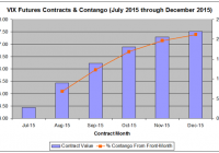
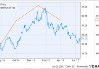
On May 19, AccuShares rolled out two new volatility ETFs–VXUP and VXDN–that were advertised to track the spot VIX without suffering the losses that plague conventional volatility ETFs like VXX. It has now been 1 month since these funds started trading and while VXUP and VXDN have achieved a portion of their objective, they have failed spectacularly in another. This article discusses the mechanics of VXUP and VXDN, compares their performance over the past month to the spot VIX and VXX, and offers alternative investment ideas. Investing in the VIX has long been a challenge for investors. Because direct investment is not possible for the average trader, an assortment of ETFs have been created to facilitate the process. The most popular of these is the iPath S&P 500 VIX Short Term Futures ETF (NYSEARCA: VXX ), although many others, including inverse and leveraged products, are also available. Unfortunately, these ETFs are all based on VIX futures contracts and inevitably underperform the VIX over the long-term, making them exceptionally difficult investments. I was therefore very excited to learn that a new pair of VIX ETFs would be entering the marketplace in mid-May that were designed to track the spot price of the VIX and to avoid futures contracts. One, the AccuShares Spot CBOE VIX UP Shares (NASDAQ: VXUP ) was designed to directly track the spot VIX while the other, the AccuShares Spot CBOE VIX DOWN Shares (NASDAQ: VXDN ) would trade inversely to the spot VIX. Could these be what volatility ETF investors have long been waiting for? It has now been one month since these new products began trading. This article analyzes the performances of VXUP and VXDN in their first month of trading and compares them to the spot VIX and VXX. VIX ETFs that use futures contracts to track the VIX are limited by the fact that VIX futures contracts expire after one month. As a result, these funds must sell their contracts by the end of each month and rotate them into the next month’s futures contract. They typically do this on a daily basis, rotating between 4% and 5% each day to rotate the entire equity of the fund in each 20- or 25-day month. Unfortunately, the VIX futures market usually trades in a steep contango, a situation where subsequent contracts are more expensive than current contracts. Figure 1 below shows the current VIX futures contracts for the next six months as of Monday’s close showing this contango. (click to enlarge) Figure 1: VIX Futures Contracts for July through December as of Monday’s close showing persistent contango with the August contrast nearly 7% more expensive than the August contract. [Source: YahooFinance ] The August 2015 futures contract is trading at a 6.8% premium to the current front month July 2015 contract. As a result, VXX is currently selling July 2015 contracts and using the funds to buy August 2015 contracts. As of Monday evening, the fund holds 82% July contracts and 18% August contracts. Over the coming weeks it will rotate 4% of its funds per day from July into August contracts. As a result, the fund is effectively selling low and buying high. Should the contango hover around 7%, the fund will suffer a daily loss of 0.04 * 0.07, or 0.28%. This is a small loss for those trading these funds on a short-term basis, but over time it adds up. Figure 2 plots VXX versus the front-month VIX contract it is designed to track over the last 1 year. (click to enlarge) Figure 2: VXX versus VIX over the past 1 year showing steep underperformance of VXX due to rollover losses. [Source: YahooFinance ] As the data above shows, VXX massively underperforms the front-month VIX futures contract, losing 41% over the last year while the VIX gained 13%. With 260 trading days, the 28% underperformance amounts to a 1-year average of 0.11% per day. This is a significant amount of drag for an investor long VXX waiting for a volatility spike. The natural gut reaction to this data would be to just short the ETF and kick back and let the profits roll in. However, this is also an inherently risky strategy. While VXX may underperform over the long-term, it can spike dramatically during market swoons. For example, during the summer of 2011 during the European Crisis, VXX jumped from $331 on July 22 to $909 on October 3, a short-breaking 174% gain. With the VIX trading at 12.74 as of Monday’s close well below its long-term average of 19 and with Greece teetering on the edge of another crisis, I would be reluctant to be short here. Due to this challenging set of trading conditions for ETFs such as VXX, investors have long clamored for an alternative ETF that did not have the limitations of futures-based VIX ETFs. Enter AccuShares. On May 19, the company released VXUP and VXDN for trading. Unlike VXX and its ilk for which the underlying index is the front month VIX Futures contracts, the underlying index for these two ETFs is the CBOE Volatility Index itself, the VIX. This should, in theory, prevent rollover losses. The management of the two is very complex. Briefly, VXUP and VXN operate as a pair and swap assets back and forth as the VIX fluctuates. Neither fund holds futures contracts, but just cash and cash equivalents such as treasuries. Each of the funds operates around a “Distribution Period” on the 15th of each month, at which point the value of the fund that gained the previous month is adjusted with payout of a cash dividend reducing its value to that of the declining fund. For example, let’s say that VXUP and VXDN each start the month out at $20/share and the VIX starts at 15. The VIX rallies 20% to 18. VXUP would be predicted to rise to $24 and VXDN would be predicted to decline to $16. At the end of this month, holders of VXUP would receive a $8 dividend in either cash or in an equal value of VXDN and the value of VXUP would be adjusted to $16, and both funds would start the next monthlong period at the same price. Finally, if the VIX is less than 30 (which it almost always is), 0.15% is transferred from VXUP to VXDN on a daily basis to provide an incentive to invest in the inverse ETF. The reasoning is that the VIX will eventually spike and investors are therefore less likely to want to buy-and-hold VXDN. At least, that is how everything is supposed to work in theory. However, this is not a discussion on the complex mechanics of these funds, but rather an analysis of their performance. Between May 19 and June 22, the VIX was remarkably flat, declining just 0.9% over the monthlong period. During the same period, VXUP declined 1.5%, a small 0.6% underperformance. VXDN gained 0.4%, a 0.5% underperformance. In contrast, VXX declined 8.8%, a much larger 7.9% underperformance. Further, VXUP and VXDN did not seen the same decay that plagues VXX and similar funds. Figure 3 below compares the monthly performance of VXUP and VXDN along with an “average” percent return between the two. If there was inherent decay and underperformance, the “average” return would be expected to steadily decline. For example, VXUP and VXDN might initially be up or down 4%, respectively, but by the end of the month would be up 8% and down 12%, respectively, for an “average” of -2%, indicating decay. (click to enlarge) Figure 3: VXUP and VXDN performance over the past month along with an average of the two showing minimal decay of the funds that would be expected of a fund based on Futures contracts such as VXX. [Source: YahooFinance ] Based on Figure 3, VXUP and VXDN trade in nearly perfect opposition over the course of the month with the average percent return between the two flat near zero indicating minimal decay. Based on these performance numbers alone, these two new ETFs look promising. However, this does not paint the entire picture. Figure 4 below plots the percent change in VXUP versus VIX over the past month. (click to enlarge) Figure 4: VXUP versus VIX over the past month showing the large volatility shortfall of VXUP compared to its underlying index. [Source: YahooFinance ] The data above shows that VXUP significantly underperformed VIX during periods of increased volatility. For example, on June 8, the VIX spiked 7.6%, but VXUP was only able to manage a 0.8% gain, barely 1/10th of the VIX’s performance. On June 15th, the VIX rallied 11.7% with VXUP gaining 3.4%, better but still an awful underperformance. Thus, the fact that VIX and VXUP both finished the month with nearly equal 1% declines is merely a function of the VIX trading flat and is unrelated to effective tracking by VXUP. To illustrate, if instead of a month range, we use the period of May 21 to June 15, the VIX gained 27% while VXUP only climbed 0.6%. In the fund’s defense, between June 15th and June 22, the VIX fell 17% while VXUP only dropped 4%. Thus, VXUP is not necessarily underperforming the VIX, it simply appears to be less volatile than the VIX. Unfortunately, volatility is what makes the VIX ETFs so popular. To analyze VXUP’s performance further, Figure 5 below shows a scatterplot of VXUP daily performance vs VIX daily performance. (click to enlarge) Figure 5: Daily performance of VIX versus VXUP over the past month showing diminished volatility of VXUP as well as mediocre tracking compared to its underlying index. [Source: YahooFinance ] This data highlights two important points, neither of which is favorable for VXUP. First, note the shallow slope of the trend line in the figure. This approximates the beta of VXUP relative to the VIX. Beta is traditionally thought of as a measure of the volatility of a security or portfolio in comparison to the market as a whole. A stock with a beta of 1 indicates that a stock’s price movement will mimic that of the market – if the S&P 500 gains 5%, the stock will gain 5%; if the market is flat, the stock will be flat; and if the market falls 5%, the stock will fall 5%. A stock with a beta of 2 is more volatile than the market – a tech stock, for example – and will gain or lose twice that of the S&P 500 or whatever index is used as the benchmark. A beta of 0.5 is comparatively less volatile – a utilities stock, for example – and will gain or lose half of the market’s performance. Betas can also be calculated for one stock or ETF versus another stock or ETF. Let’s calculate the beta for VXUP relative to VIX. If the Beta is 1, this means that VXUP sees daily gains and losses comparable to that of the VIX. We already know what the result is going to be. Unfortunately, the beta for VXUP over the past month has been 0.21, meaning that the fund is only about 1/5th as volatile as the index it is trying to track. In other words, its creators successfully sought to eliminate decay and underperformance, but eliminated all-important volatility and opportunity for outsized gains that makes VIX products so popular investors. Second, Figure 5 also shows that VIX and VXUP don’t really correlate all that well as there is significant scattering around the trend line. The R^2 for the relationship is a lackluster 0.68 indicating a poor day-to-day tracking. In fact, VXUP isn’t all that much better than an ordinary Index ETF, both in terms of approximating the volatility of the VIX and effectively tracking its day-to-day movement. Let’s perform the same calculation as in Figure 5 using the SPDR S&P 500 ETF Trust (NYSEARCA: SPY ), the oldest and most popular index ETF, instead of VXUP. A scatterplot comparing daily movement of VIX versus SPY is shown below in Figure 6. (click to enlarge) Figure 6: Daily performance of VIX versus SPY over the past month showing comparable volatility of SPY and VXUP (shown in Figure 5). [Source: YahooFinance ] Note that SPY actually tracks the VIX more accurately on a daily basis than VXUP with an R^2 value of 0.79 vs 0.68 for VXUP, although of course the relationship between the two is inverse in that SPY goes down when the VIX goes up. The beta for SPY to the VIX is -0.08 compared to 0.21 for VXUP indicating similar levels of volatility. If one wanted to approximate VXUP’s volatility even more closely using an index ETF, a trader could go long the inverse leveraged Direxion Daily S&P 500 Bear 3x ETF (NYSEARCA: SPXS ) which has a beta of 0.23 and an R^2 of 0.80 relative to the VIX, beating VXUP on both fronts. What conclusions can be drawn from this data? On the one hand, VXUP and VXDN have, after 1 month, avoided the decay from rollover losses that plague Futures-based VIX ETFs like VXX. However, the ETFs have come up woefully short in tracking the day-to-day performance of the spot VIX and matching its volatility, which is what they were advertised to do. In fact, if a trader wants to be free of the rollover-induced decay seen in VXX and approximate the level of volatility seen in VXUP over the past month, he or she is better of shorting a simple index fund such as SPY or buying an inverse index ETF such as SPXS as these have better daily tracking than VXUP and comparable levels of volatility. To be compared to an index fund–intended to be a stable, non-volatile long-term investment for those actively trying to AVOID volatility seen in individual stocks–is a giant slap in the face for a volatility ETF. To put it more succinctly: I want volatility with my volatility ETF! Yes, the funds outperformed VXX, although this could be said of most index ETFs last month. Were the VIX to have spiked, VXX would have likely outperformed VXUP by a considerable margin. While I would like to give these funds the benefit of the doubt that perhaps they will more accurately track the VIX should it start trending directionally rather than the chop that we saw last month, I consider them to be failed funds right now. It is one thing for a fund like VXX to underperform its underlying commodity. Traders know why it does so and accept that underperformance as the cost of the opportunity for volatility exposure. VXUP/VXDN, on the other hand, are more than five-fold less volatile than expected, and it is not clear why. AccuShares had announced plans for similar paired funds for oil, natural gas, metals, and agricultural commodities, but I expect these ETFs will be tabled for now. Where does this leave us? To be honest, I believe trying to get long the VXX is a fool’s errand. Too much comes down to timing. VXX may track the VIX much better than VXUP–it has a beta of 0.41 with an R^2 of 0.89 relative to VIX–but it is suffers the rollover-induced drag discussed above. While the VIX will inevitably spike, waiting for it to do so long VXX can be very costly and not only holds your funds captive, but the eventual volatility spike might not even be enough to overcome rollover losses. The only situation in which I would consider going long VXX would be if the VIX were less than 12, more than 2 standard deviations below its long-term average. Over the last 25 years, when the VIX is less than 12, it rallies an average of 13% over the following month, rising 79% of the time, a high probability jump with a large enough magnitude that would likely outweigh any rollover-induced losses. With the VIX closing at 12.74 on Monday, we may actually be approaching this level. At the same time, I would be very reluctant to short VXX at these levels, even with a 6% monthly drag due to contango given the increased probability of a volatility spike. I prefer the higher probability play and would only consider shorting VXX if the VIX climbed above 20, which would limit further upside risk and allow profits both from rollover losses and any mean-reversion that takes place as volatility subsides. In the meantime, I believe that there are much better investments out there that do not come with the same risks as VXX or the limitations of VXUP. In conclusion, VXUP and VXDN were an admirable attempt by AccuShares to create a novel volatility product that was not dependent on VIX futures contracts and the disadvantages that come with these contracts. However, to date, it has failed to even come close to meeting its objective of tracking the spot VIX on a daily basis. The volatility of VXUP to date is so underwhelming that an investor would just as well use index funds to achieve the same level of volatility exposure. Therefore, I plan to avoid these ETFs barring a significant improvement in daily volatility. That being said, I am not enamored with the alternatives either. While VXX is roughly twice as volatile as VXUP, it’s rollover-induce losses drain a portfolio while waiting for a spike in voltility. Put another way, VXUP and VXDN remove some of the risk of volatility ETFs but take away most of the reward. VXX has more potential for reward, but introduces extra risk in the form of rollover losses. I would only recommend going long VXX when the VIX is at historical lows. Likewise, I would only take advantage of the rollover-induced losses and short the VXX when the VIX is elevated above its baseline average to reduce the risk of a spike in volatility that would devastate a short position. In the meantime, there are over 4000 actively traded stocks in the NYSE and Nasdaq. There are at least a couple that are better bets than trying to force the issue with volatility right now. Disclosure: I/we have no positions in any stocks mentioned, and no plans to initiate any positions within the next 72 hours. (More…) I wrote this article myself, and it expresses my own opinions. I am not receiving compensation for it (other than from Seeking Alpha). I have no business relationship with any company whose stock is mentioned in this article.

Warm Weather In Q1 Didn’t Diminish Portland General Electric’s Long-Term Outlook

Summary Utility Portland General Electric’s Q1 earnings were dampened by unseasonably warm weather in Q1, which caused its sales volume to decline and earnings to miss the consensus estimate. The company would have had a solid quarter but for the mild winter, however, and it benefited from low fuel costs and a growing customer base. Weather aside, the company has continued to invest heavily in new non-coal capacity that will allow it to take full advantage of expected strong employment growth in its service area. While its shares appear to be undervalued at present, I would prefer to wait for them to fall to $31, a move that could occur with rising interest rates. Western electric utility Portland General Electric (NYSE: POR ) saw its share price approach a 52-week low earlier this month in the wake of a disappointing Q1 earnings report and subsequent downgrade by J.P. Morgan . While weather-related issues did negatively impact the company’s earnings earlier in the year, its trailing EBITDA is just short of a 15-year high (see figure). Furthermore, a disappointing short-term operating outlook co-exists with a more optimistic long-term outlook. This article evaluates Portland General Electric as a long-term investment in light of its recent performance and operating outlook. POR data by YCharts Portland General Electric at a glance Portland General Electric generates and distributes electricity from a number of fossil and renewable sources in the state of Oregon. The company’s most recent public iteration (its history as a firm dates to the late 19th century) came after it was divested from Enron in 2006 following the latter’s bankruptcy. Portland General Electric distributes electricity to 44% of Oregon’s inhabitants, with a total of 841,000 customers throughout the state, including much of the city of Portland (it divides service to the eponymous city with Berkshire Hathaway subsidiary Pacific Power ). The majority of Portland General Electric’s existing generating capacity , or 2,139 MW, comes from thermal power, split between roughly 65% natural gas and 35% coal. The company also utilizes substantial renewable sources, however, including 717 MW of wind power and 501 MW of hydroelectric power. A further 100 MW is purchased from third parties and resold by the firm. Oregon has recently begun to push companies in the state toward the replacement of fossil fuels with renewable resources, as evidenced by its March 2015 adoption of a low-carbon fuel standard. While the new standard is limited to transportation fuels, its implementation has led to proposals for the state to further adopt a carbon tax on fossil fuels, including fossil-based electricity. Recognizing the new trend, Portland General Electric will have phased out 61% of its coal-based capacity (i.e., its Boardman coal-fired facility) by 2020. As part of this effort the company is exploring the replacement of this capacity with biomass in a move that would create one of the largest biomass power facilities in the country. In the meantime it is building a new 440 MW natural gas-fired facility next to the existing Boardman coal-fired facility, thereby ensuring that its overall capacity will not be adversely affected by the closure of the coal-fired facility even in the event that biomass is not determined to be a feasible alternative feedstock. Portland General Electric is also moving forward with regulatory assessments of a new planned 6 MW hydroelectric dam in the state. As with other regulated electric utilities, Portland General Electric’s trailing earnings have been relative stable (see table). The most recent five quarters have been a strong rebound from 2013, however, when the company’s net income and EBITDA fell sharply. Overall it has been a consistent performer, however, reporting quarterly net losses on just two occasions in the nine years since it separated from Enron. As a regulated utility the company is dependent on state regulators to set rates at a level that will allow it to cover its cost of capital, and past earnings volatility has often been a result of regulators setting rates at levels below those requested by the company (the most recent example being the 2015 rates). Despite this most recent disappointment, however, Portland General Electric still manages to boast trailing net margin, return on equity, and return on assets figures that exceed the industry average. Portland General Electric Financials (non-adjusted) Q1 2015 Q4 2014 Q3 2014 Q2 2014 Q1 2014 Revenue ($MM) 473.0 500.0 484.0 423.0 493.0 Gross income ($MM) 250.0 239.0 222.0 214.0 255.0 Net income ($MM) 50.0 43.0 39.0 35.0 58.0 Diluted EPS ($) 0.62 0.52 0.47 0.43 0.73 EBITDA ($MM) 160.0 160.0 153.0 141.0 173.0 Source: Morningstar (2015) Portland General Electric also maintains relatively little cash on its balance sheet, with this amount falling to only $27 million at the end of Q1 (see table), relying instead upon steady operating cash flow and cheap credit to cover its substantial capital expenditures. At the end of Q1 the company listed $483 million in cash including short-term credit and letter of credit capacity maturing in November 2019. Furthermore, while it had an additional $2.1 billion in long-term debt at the end of the quarter, this was available at low rates (3.5% on 15-year debt, for example). While the company’s current ratio of 0.72 and substantial long-term debt load would be a cause for concern in other industries, Portland General Electric has no difficulty in acquiring additional financing as needed. Furthermore, its recent record of negative free cash flow has been the result of its large investments in additional capacity to meet demand growth in its service area, and these should pay substantial dividends (both figuratively and literally) as it comes online in 2017 and 2018. Portland General Electric Balance Sheet (restated) Q1 2015 Q4 2014 Q3 2014 Q2 2014 Q1 2014 Total cash ($MM) 27.0 127.0 97.0 97.0 64.0 Total assets ($MM) 7,091.0 7,042.0 6,657.0 6,399.0 6,169.0 Current liabilities ($MM) 809.0 873.0 482.0 457.0 451.0 Total liabilities ($MM) 5,152.0 5,131.0 4,768.0 4,528.0 4,313.0 Source: Morningstar (2015). Q1 earnings report Portland General Electric reported disappointing earnings in late April for Q1, missing on both lines. Revenue came in at $473 million, down 4.1% YoY from $493 million and missing the consensus estimate by $17.3 million. The company attributed the poor result to a substantial decline to sales volumes resulting from an unseasonably warm winter in its service area. Heating degree days in Q1 were down 21.7% from the previous year and 20% from the 15-year average, reducing demand as its customers were not forced to turn their heaters on as frequently as usual. The Q1 sales volume fell by 3.5% YoY, reducing revenue by $16 million. The company reported net income of $50 million, down from $58 million the previous year. Diluted EPS was $0.62 compared to $0.73 YoY, missing the consensus estimate by $0.10. EBITDA fell to $160 million from $173 million YoY. The company stated that diluted EPS would have been higher by $0.20 had the number of heating degree days for the quarter matched the 15-year average, while the expiration of the Production Tax Credit for wind power and abnormally low wind supply in the quarter reduced EPS by another $0.08. Partially offsetting these reductions was the sharp fall in the prices of natural gas and coal that occurred in the second half of 2014, which reduced the company’s operating costs by $23 million. Generation, transmission, and distribution costs rose 15% YoY but this was due to new capacity coming online. Finally, the company increased its number of retail customers by 0.7% YoY. But for the weather, then, Q1 would have been a solid quarter for the company. Indeed, the company’s management was confident enough in its overall performance to increase the quarterly dividend by 7% from $0.28 to $0.30 a week after the earnings report’s release, bringing its forward yield to a respectable 3.5%. Outlook Portland General Electric reported during its Q1 earnings call that its expansion plans are moving ahead as intended. The aforementioned new 440 MW Boardman natural gas-fired facility is on schedule to be mechanically completed by Q2 2016 and is on track to meet its estimated budget of $450 million. Its gas turbine and generator were installed in Q1 and its steam generator is expected to be constructed this quarter, bringing its overall construction to 50% completion. The company intends to finance its future capital expenditures, which could exceed $2.5 billion through 2018, via its operating cash flow ($494 million TTM), $400 million in new debt, and $270 million from equity forward sales that are due to be completed by the end of Q2. Finally, the company has requested a net 3.7% customer price increase for FY 2016 and expects state regulators to issue a decision by the end of 2015. Investors should note that the regulators have a history of awarding Portland General Electric lower-than-requested rate increases, however. Management stated in its Q1 earnings call that it is reducing its FY 2015 diluted EPS guidance from $2.20-$2.35 to $2.05-$2.20 in response to the weather-induced Q1 earnings miss. Beyond 2015, however, there are reasons to expect the company’s earnings to rebound. First, its Q1 earnings would have been stronger but for the quarter’s unseasonably warm weather. A return to the long-run average next year, let alone a colder-than-average winter such as the Northeast U.S. experienced at the same time, would provide its earnings with a boost. Similarly, the warm weather contributed to a record-low snowpack in Oregon that reduced the electricity yielded from Portland General Electric’s sizeable hydroelectric capacity, forcing it to increase its reliance on purchased power rather than its own generators. While there is no guarantee that next winter will provide a more favorable operating environment for the company, the 15-year average suggests that it will. Portland General Electric also benefits from operating in a state that has seen its labor rolls grow faster than the U.S. average since 2013 in a trend that is forecast to become particularly pronounced after 2017 (see figure). The company’s heavy investment in new capacity will, if the forecasts turn out to be correct, allow it to take full advantage of this trend by adding new customers and responding to increases in existing demand as economic growth strengthens still further. While its limited geographic exposure has been a burden at times in the past, Oregon’s expected above-average economic growth will similarly provide the company with an advantage over utilities in other parts of the country in coming years. Indeed, it could even make Portland General Electric a possible takeover target, although such an event is too speculative at present to have a large influence on an investment decision. Oregon Total Nonfarm Employment data by YCharts Finally, Portland General Electric can also be expected to benefit from last year’s sharp decline in the price of natural gas. While the fall hasn’t been as pronounced in Oregon as in the central and south-central U.S., the state is still experiencing citygate prices that are 21% lower today than at the same time a year ago (see figure). Continued low natural gas prices will provide the company with a couple of advantages. First, it places it in a position to take advantage of low prices and potentially invest in the acquisition of large natural gas reserves that can be utilized if and when prices increase in the future. Management stated during the Q1 earnings call that it is actively exploring such an investment, and I would expect to see the company move forward with it in the event that natural gas prices fall much further. Second, cheap natural gas increases the feasibility and reduces the opportunity costs of its move away from coal-fired facilities. Natural gas has less than half of the carbon intensity of coal when used to produce electricity and a switch from the latter to the former will both boost the company’s public image and mitigate the adverse impact of a possible carbon tax in the state. Oregon Natural Gas Citygate Price data by YCharts Valuation Not surprisingly, analyst estimates for FY 2015 have been revised lower over the last 60 days in response to management’s own lowered guidance. The diluted EPS consensus estimate for FY 2015 has fallen from $2.29 to $2.16, although the FY 2016 estimate has remained steady over the same period at $2.39. Based on the share price at the time of writing of $34.29, the company has a trailing P/E ratio of 16.8x. The consensus estimates result in forward ratios for FY 2015 and FY 2016 of 15.9x and 14.3x, respectively. While the trailing ratio is high compared to its 3-year history (see figure), the forward ratios are relatively low. POR PE Ratio (NYSE: TTM ) data by YCharts Conclusion Portland General Electric reported disappointing earnings for Q1 due to unseasonably warm conditions and investors have pushed the company’s shares near their 52-week low in response. While there are no guarantees that future weather conditions will be more favorable, even a return to the long-run average conditions would provide the company’s future earnings with a substantial boost. Beyond the current fiscal year, the company is continuing to invest heavily in new generating capacity, both as part of a move away from coal as well as in response to expectations of increased demand over the next several years as Oregon’s employment growth is forecast to substantially exceed that of the U.S. While Portland General Electric does not benefit from as friendly of a relationship with state regulators as many of its competitors do, I ultimately believe that this is outweighed by its geographic location and generating capacity investments. The only thing that prevents me from initiating a long investment at this time is the prospect of rising interest rates later in the year and movement of large investors away from utilities and other dividend stocks. I believe that the company’s share price could follow those of other dividend stocks lower in anticipation of a rate rise later in the year. Following such a decline, however, I would readily purchase Portland General Electric’s shares for $31, or approximately 13x its expected FY 2016 earnings. Disclosure: I/we have no positions in any stocks mentioned, and no plans to initiate any positions within the next 72 hours. (More…) I wrote this article myself, and it expresses my own opinions. I am not receiving compensation for it (other than from Seeking Alpha). I have no business relationship with any company whose stock is mentioned in this article.

Is GREK Today’s Least Competitive Wealth-Builder ETF Investment?

Summary Days ago our article identified an ETF ranked at the best end of the scale posed in the title above, drawing Seeking Alpha reader attention. The ongoing EU vs. Greece drama now reaching a moment of (possible) truth has as one (or more) possible outcome(s) capable of defining an immediate tragedy. Hence the question being raised. And if this is not the worst possible choice of a long ETF position, is (are) there more threatening one(s)? Market-makers have to appraise them all, to do their jobs. We use their hedging actions to tell us what they think. It’s beyond our ken. Way beyond. Value analysis requires comparisons. Without appraisal of the bad, how do we know good? Yin and Yang are both essential. How does GREK look to market-makers? The Global X FTSE Greece 20 ETF (NYSEARCA: GREK ) presents market-makers with a challenging task of appraisal. In our recent article we posed the question this way: From a population of some 350 actively-traded, substantial, and growing ETFs is this a currently attractive addition to a portfolio whose principal objective is wealth accumulation by active investing? We daily evaluate future near-term price gain prospects for quality, market-seasoned ETFs, based on the expectations of market-makers [MMs], drawing on their insights from client order-flows. Following that article’s format where possible, let’s look at their appraisal of GREK. Yahoo describes it this way: The fund currently holds assets of $310 million and has had a YTD price return of -9.1%. Its average daily trading volume of 899,906 produces a complete asset turnover calculation in 29 days at its current price of $11.77. (The Bank of Piraeus may wish it had as long on withdrawals.) Behavioral analysis of market-maker hedging actions while providing market liquidity for volume block trades in the ETF by interested major investment funds has produced the recent past (6 month) daily history of implied price range forecasts pictured in Figure 1. Figure 1 (used with permission) The vertical lines of Figure 1 are a visual history of forward-looking expectations of coming prices for the subject ETF. They are NOT a backward-in-time look at actual daily price ranges, but the heavy dot in each range is the ending market quote of the day the forecast was made. What is important in the picture is the balance of upside prospects in comparison to downside concerns. That ratio is expressed in the Range Index [RI], whose number tells what percentage of the whole range lies below the then current price. Today’s Range Index is used to evaluate how well prior forecasts of similar RIs for this ETF have previously worked out. The size of that historic sample is given near the right-hand end of the data line below the picture. The current RI’s size in relation to all available RIs of the past 5 years is indicated in the small blue thumbnail distribution at the bottom of Figure 1. The first items in the data line are current information: The current high and low of the forecast range, and the percent change from the market quote to the top of the range, as a sell target. The Range Index is of the current forecast. Other items of data are all derived from the history of prior forecasts. They stem from applying a T ime- E fficient R isk M anagement D iscipline to hypothetical holdings initiated by the MM forecasts. That discipline requires a next-day closing price cost position be held no longer than 63 market days (3 months) unless first encountered by a market close equal to or above the sell target. The net payoffs are the cumulative average simple percent gains of all such forecast positions, including losses. Days held are average market rather than calendar days held in the sample positions. Drawdown exposure indicates the typical worst-case price experience during those holding periods. Win odds tells what percentage proportion of the sample recovered from the drawdowns to produce a gain. The cred(ibility) ratio compares the sell target prospect with the historic net payoff experiences. Figure 2 provides a longer-time perspective by drawing a once-a week look from the Figure 1 source forecasts, back over (almost) two years. Figure 2 (used with permission) What does this ETF hold, causing such price expectations? Figure 3 is a table of securities held by the subject ETF, indicating its concentration in the top ten largest holdings, and their percentage of the ETF’s total value. Figure 3 (click to enlarge) Well, maybe that’s what is causing such price expectations, but it seems more likely that international politics has more to do with it. So let’s depart from GRKZF, the Greek Organization of Football Prognostics SA, and turn to the Wall Street organization of stock price prognostics, or market-makers [MMs]. Sport is where you find it. Just how bad is the GREK outlook? We use the MMs forecasts for stock and ETF prices, implied by their self-protective hedging actions, plus the accumulated actuarial history of market price events following such prior forecasts as are seen today, to rank each subject. Figure 4 is a table of how the worst-ranking ten ETFs appear. Please remember, our ranking interest is in wealth-building, not wealth destruction. What works well in one direction may not work in the opposite. Shorting is not recommended. Figure 4 (click to enlarge) When we compare the wealth-building prospects for GREK (ranked 270th out of 340) it doesn’t come close to the terrors inherent in these last ten. Remember, the MMs role is to build a balance between buyers and sellers in every trade, so they have to find acceptable expectations at each end of an actionable array of prices. The actions produce the trade, the expectations are what produce the actions. Check the row of data beneath the top illustration of Figure 1. Its forecast upper end is 23.7% above the then-current price of $10.58. That compares to the ten-ETF average of Figure 4 of +29.4% in column (5). What of the risk exposure? When GREK in the past has been seen by MMs to have an outlook like today’s (a Range Index of 33, meaning twice as much upside as downside) its typical worst-case price drawdown experienced was but -16.3%. The worst-ten ETFs of Figure 4 managed -19.7% — a fifth of their capital gone, not just less than a sixth. And on top of that GREK had 42 out of 100 chances of seeing its price recover back into profit territory, while those other ETFs had but one chance in four of that happening (column 8 blue average). And they started, on average, from prior forecasts with Range Indexes of 26, with three times as much upside as down. See? GREK could be worse. ‘Course it could (needs to) be better. The average equity today offers a 29 Range Index with +12.5% upside. There is real credibility to that population forecast, since prior similar forecast hypothetical positions produced gains of +3.9% (net of 35/100 losses, not 58/100). GREK actually had prior net losses of -6.5% and negative credibility ratio (like the other worst ten ETFs) comparing upside forecasts to actual TERMD payoffs. Conclusion But those are historical comparisons. The past may not be prologue. Buyers must hope so. Besides, there is less than two years of GREK pricing for us to work with. Maybe Greece has just had a bad recent two years. We keep a ten-foot long pole at hand for just such occasions. Hope we don’t have to use it, not sure we would. Disclosure: I/we have no positions in any stocks mentioned, and no plans to initiate any positions within the next 72 hours. (More…) I wrote this article myself, and it expresses my own opinions. I am not receiving compensation for it (other than from Seeking Alpha). I have no business relationship with any company whose stock is mentioned in this article.