Tag Archives: seeking

Industrial ETF: XLI No. 6 Select Sector SPDR In 2014

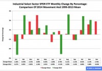
Summary The Industrial exchange-traded fund finished sixth by return among the nine Select Sector SPDRs in 2014. The ETF was especially strong in the fourth quarter of last year, when it advanced 7.06 percent. However, seasonality analysis indicates the fund could be weak in the first quarter of this year. The Industrial Select Sector SPDR ETF (NYSEARCA: XLI ) in 2014 ranked No. 6 by return among the Select Sector SPDRs that cut the S&P 500 into nine sections. On an adjusted closing daily share-price basis, XLI grew to $56.58 from $51.27, an increase of $5.31, or 10.36 percent. Therefore, it trailed its sibling, the Utilities Select Sector SPDR ETF (NYSEARCA: XLU ), and parent proxy, the SPDR S&P 500 Trust ETF (NYSEARCA: SPY ) by -18.38 and -3.11 percentage points, in that order. (XLI closed at $54.93 Tuesday.) XLI also ranked No. 6 among the sector SPDRs in the fourth quarter, when it behaved better than SPY by 2.16 percentage points and worse than XLU by -6.13 points. And XLI ranked No. 4 among the sector SPDRs in December, when it led SPY by 0.23 percentage point and lagged XLU by -3.59 points. Figure 1: XLI Monthly Change, 2014 Vs. 1999-2013 Mean (click to enlarge) Source: This J.J.’s Risky Business chart is based on analyses of adjusted closing monthly share prices at Yahoo Finance . XLI behaved better in 2014 than it did during its initial 15 full years of existence based on the monthly means calculated by employing data associated with that historical time frame (Figure 1). The same data set shows the average year’s weakest quarter was the third, with a relatively small negative return, and its strongest quarter was the fourth, with an absolutely large positive return. Consistent with this pattern last year, the ETF had a small loss in Q3 and a large gain in Q4. Figure 2: XLI Monthly Change, 2014 Versus 1999-2013 Median (click to enlarge) Source: This J.J.’s Risky Business chart is based on analyses of adjusted closing monthly share prices at Yahoo Finance. XLI performed worse in 2014 than it did during its initial 15 full years of existence based on the monthly medians calculated by using data associated with that historical time frame (Figure 2). The same data set shows the average year’s weakest quarter was the third, with an absolutely large positive return, and its strongest quarter was the fourth, with an absolutely larger positive return. It also shows there is a historical statistical tendency for the ETF to struggle in January. Figure 3: XLI’s Top 10 Holdings and P/E-G Ratios, Jan. 13 (click to enlarge) Note: The XLI holding-weight-by-percentage scale is on the left (green), and the company price/earnings-to-growth ratio scale is on the right (red). Source: This J.J.’s Risky Business chart is based on data at the XLI microsite and FinViz.com (both current as of Jan. 13). The World Bank Group became the latest economic observer to offer evidence of a slowdown in the growth of gross domestic product on this planet in the Global Economic Prospects report it released Tuesday. In its most recent semiannual report, the international financial institution based in Washington estimated GDP grew 2.6 percent in 2014, compared with its forecasts of 2.8 percent last June and 3.2 percent last January: Global growth in 2014 was lower than initially expected, continuing a pattern of disappointing outturns over the past several years. Growth picked up only marginally in 2014, to 2.6 percent, from 2.5 percent in 2013. Beneath these headline numbers, increasingly divergent trends are at work in major economies. While activity in the United States and the United Kingdom has gathered momentum as labor markets heal and monetary policy remains extremely accommodative, the recovery has been sputtering in the euro area and Japan as legacies of the financial crisis linger, intertwined with structural bottlenecks. China, meanwhile, is undergoing a carefully managed slowdown. Disappointing growth in other developing countries in 2014 reflected weak external demand, but also domestic policy tightening, political uncertainties and supply-side constraints. In its GEP report, the World Bank also cut its forecasts of GDP growth in 2015, to 3.0 percent from 3.4 percent, and in 2016, to 3.3 percent from 3.5 percent. The conditions underlying these cuts in the World Bank’s forecasts appear likely to have deleterious effects on the earnings of many of XLI’s constituent companies (i.e., those with major exposures to the global economy). This is especially so given the bias divergence in monetary policy at major central banks around the world and its impact on currency-exchange rates, as discussed in “PowerShares QQQ’s 2014 And Fourth-Quarter Performance And Seasonality.” At this late stage of the economic/market cycle, the valuations of XLI’s top 10 and other holdings seem unlikely to function as tailwinds for the ETF’s price appreciation in the foreseeable future (Figure 3). However, the numbers on the S&P 500 industrial sector reported by S&P Senior Index Analyst Howard Silverblatt Dec. 31 suggest it is not hideously overvalued, with its P/E-G ratio at 1.37: not cheap to the likes of me, not dear to the likes of normal people. Disclaimer: The opinions expressed herein by the author do not constitute an investment recommendation, and they are unsuitable for employment in the making of investment decisions. The opinions expressed herein address only certain aspects of potential investment in any securities and cannot substitute for comprehensive investment analysis. The opinions expressed herein are based on an incomplete set of information, illustrative in nature, and limited in scope. In addition, the opinions expressed herein reflect the author’s best judgment as of the date of publication, and they are subject to change without notice.

DGRW Is A Solid ETF In Every Metric, But Still Faces An Uphill Battle

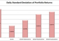
Summary I’m taking a look at DGRW as a candidate for inclusion in my ETF portfolio. The risk level on the ETF looks good with heavy trading volume. The yield is lower than I would expect for an ETF focused on dividend growth. The exposure to oil companies might be a bit much when I’m also planning a portion of my portfolio for natural resources. I’m not assessing any tax impacts. Investors should check their own situation for tax exposure. How to read this article : If you’re new to my ETF articles, just keep reading. If you have read this intro to my ETF articles before, skip down to the line of asterisks. This section introduces my methodology. By describing my method initially, investors can rapidly process each ETF analysis to gather the most relevant information in a matter of minutes. My goal is to provide investors with immediate access to the data that I feel is most useful in making an investment decision. Some of the information I provide is readily available elsewhere, and some requires running significant analysis that, to my knowledge, is not available for free anywhere else on the internet. My conclusions are also not available anywhere else. What I believe investors should know My analysis relies heavily on Modern Portfolio Theory. Therefore, I will be focused on the statistical implications of including a fund in a portfolio. Since the potential combinations within a portfolio are practically infinite, I begin by eliminating ETFs that appear to be weak relative to the other options. It would be ideal to be able to run simulations across literally billions of combinations, but it is completely impractical. To find ETFs that are worth further consideration I start with statistical analysis. Rather than put readers to sleep, I’ll present the data in charts that only take seconds to process. I include an ANOVA table for readers that want the deeper statistical analysis, but readers that are not able to read the ANOVA table will still be able to understand my entire analysis. I believe there are two methods for investing. Either you should know more than the other people performing analysis so you can make better decisions, or use extensive diversification and math to outperform most investors. Under CAPM (Capital Asset Pricing Model), it is assumed every investor would hold the same optimal portfolio and combine it with the risk free asset to reach their preferred spot on the risk and return curve. Do you know anyone that is holding the exact same portfolio you are? I don’t know of anyone else with exactly my exposure, though I do believe there are some investors that are holding nothing but SPY . In general, I believe most investors hold a portfolio that has dramatically more risk than required to reach their expected (under economics, disregarding their personal expectations) level of returns. In my opinion, every rational investor should be seeking the optimal combination of risk and reward. For any given level of expected reward, there is no economically justifiable reason to take on more risk than is required. However, risk and return can be difficult to explain. Defining “Risk” I believe the best ways to define risk come from statistics. I want to know the standard deviation of the returns on a portfolio. Those returns could be measured daily, weekly, monthly, or annually. Due to limited sample sizes because some of the ETFs are relatively new, I usually begin by using the daily standard deviation. If the ETF performs well enough to stay on my list, the next levels of analysis will become more complex. Ultimately, we probably shouldn’t be concerned about volatility in our portfolio value if the value always bounced back the following day. However, I believe that the vast majority of the time the movement today tells us nothing about the movement tomorrow. While returns don’t dictate future returns, volatility over the previous couple years is a good indicator of volatility in the future unless there is a fundamental change in the market. Defining “Returns” I see return as the increase over time in the value known as “dividend adjusted close”. This value is provided by Yahoo. I won’t focus much on historical returns because I think they are largely useless. I care about the volatility of the returns, but not the actual returns. Predicting returns for a future period by looking at the previous period is akin to placing a poker bet based on the cards you held in the previous round. Defining “Risk Adjusted Returns” Based on my definitions of risk and return, my goal is to maximize returns relative to the amount of risk I experienced. It is easiest to explain with an example: Assume the risk free rate is 2%. Assume SPY is the default portfolio. Then the risk level on SPY is equal to one “unit” of risk. If SPY returns 6%, then the return was 4% for one unit of risk. If a portfolio has 50% of the risk level on SPY and returns 4%, then the portfolios generated 2% in returns for half of one unit of risk. Those two portfolios would be equal in providing risk adjusted returns. Most investors are fueled by greed and focused very heavily on generating returns without sufficient respect for the level of risk. I don’t want to compete directly in that game, so I focus on reducing the risk. If I can eliminate a substantial portion of the risk, then my returns on a risk adjusted basis should be substantially better. Belief about yields I believe a portfolio with a stronger yield is superior to one with a weaker yield if the expected total return and risk is the same. I like strong yields on portfolios because it protects investors from human error. One of the greatest risks to an otherwise intelligent investor is being caught up in the mood of the market and selling low or buying high. When an investor has to manually manage their portfolio, they are putting themselves in the dangerous situation of responding to sensationalistic stories. I believe this is especially true for retiring investors that need money to live on. By having a strong yield on the portfolio it is possible for investors to live off the income as needed without selling any security. This makes it much easier to stick to an intelligently designed plan rather than allowing emotions to dictate poor choices. In the recent crash, investors that sold at the bottom suffered dramatic losses and missed out on substantial gains. Investors that were simply taking the yield on their portfolio were just fine. Investors with automatic rebalancing and an intelligent asset allocation plan were in place to make some attractive gains. Personal situation I have a few retirement accounts already, but I decided to open a new solo 401K so I could put more of my earnings into tax advantaged accounts. After some research, I selected Charles Schwab as my brokerage on the recommendation of another analyst. Under the Schwab plan “ETF OneSource” I am able to trade qualifying ETFs with no commissions. I want to rebalance my portfolio frequently, so I have a strong preference for ETFs that qualify for this plan. Schwab is not providing me with any compensation in any manner for my articles. I have absolutely no other relationship with the brokerage firm. Because this is a new retirement account, I will probably begin with a balance between $9,000 and $11,000. I intend to invest very heavily in ETFs. My other accounts are with different brokerages and invested in different funds. Views on expense ratios Some analysts are heavily opposed to focusing on expense ratios. I don’t think investors should make decisions simply on the expense ratio, but the economic research I have covered supports the premise that overall higher expense ratios within a given category do not result in higher returns and may correlate to lower returns. The required level of statistical proof is fairly significant to determine if the higher ratios are actually causing lower returns. I believe the underlying assets, and thus Net Asset Value, should drive the price of the ETF. However, attempting to predict the price movements of every stock within an ETF would be a very difficult and time consuming job. By the time we want to compare several ETFs, one full time analyst would be unable to adequately cover every company. On the other hand, the expense ratio is the only thing I believe investors can truly be certain of prior to buying the ETF. Taxes I am not a CPA or CFP. I will not be assessing tax impacts. Investors needing help with tax considerations should consult a qualified professional that can assist them with their individual situation. The rest of this article By disclosing my views and process at the top of the article, I will be able to rapidly present data, analysis, and my opinion without having to explain the rationale behind how I reached each decision. The rest of the report begins below: ******** (NASDAQ: DGRW ) WisdomTree U.S. Dividend Growth Fund Tracking Index: WisdomTree U.S. Dividend Growth Index Allocation of Assets: 80% Invested in components of the index or other securities that are considered to be almost identical Morningstar Category: Large Blend Time period starts: June 2013 Time period ends: December 2014 Portfolio Std. Deviation Chart: (click to enlarge) (click to enlarge) Returns over the sample period: (click to enlarge) Correlation: 96.34 Liquidity: 498,146 average shares/day Days with no change in dividend adjusted close: 10 Yield: 1.77% Expense Ratio: .28% Discount or Premium to NAV: .23% premium Holdings: (click to enlarge) Further Consideration: Yes. I am planning to allocate a portion of my portfolio to focus on dividend growth stocks because I want them to be over-weighted in my portfolio. Conclusion: DGRW doesn’t offer much in the way of diversification with a correlation that is over 96% and 10 days with no change in dividend adjusted close. There were only 2 days where SPY reported no change in dividend adjusted close during the same period. DGRW having 10 days rather than 2 may simply be a rounding error because DGRW trades around $31 to $32 and SPY is trading at over $200. A one cent movement in DGRW is similar to a six cent movement in SPY. The liquidity based on shares/day combined with the relatively low standard deviation results in an ETF that should fit nicely into portfolios that are requiring some liquidity. However, the distribution yield of 1.77% (lower than SPY’s 1.87%) is interesting for an ETF that suggests dividends are a primary focus. The expense ratio isn’t too bad and wouldn’t be enough to scare off, though I would prefer to buy closer to NAV since I expect to rebalance frequently which makes spreads and premiums or discounts more important to my strategy. With this much liquidity I would expect spreads to remain fairly small whenever the market is open and I would expect the premiums to disappear fairly fast. My biggest concern on this ETF would probably be the concentration of holdings. I don’t mind having a large position in Exxon Mobil, but I may be creating that position through an ETF that focuses on exposure to natural resources. Since I intend to include sections for a replacement for SPY and an allocation to an ETF that focuses on dividends, there will naturally be some significant exposure coming from three ETFs, but I’d like to keep the company specific risk as low as possible so that no company can compose more than 2 to 3% of my portfolio. Since the yield on the ETF is relatively low and it substantially overlaps with other positions I intend to create, I think it will face a slightly uphill battle despite being attractive ETF. As shown from the ending Portfolio Value, the high correlation also has a very similar total return. That isn’t always the case when using daily standard deviation, but it has been the case for DGRW. Comments I’m testing a new layout for my ETF articles. It is intended to optimize the articles for my followers. Let me know what you think of the new layout in the comments section. I’m always looking for feedback and trying to find ways to improve my writing for my readers.
Atlanta Fed Lockhart Ambiguity And GLD

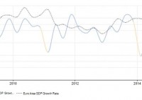
Summary Lockhart will be a new voting FOMC member this year and his first speech of 2015 starts off with a bullish note which justifies rates normalization. Strategic ambiguity of rate hikes in the middle of the year and Lockhart worries about mixed signals in first half of 2015. On mixed reading and to be on the safe side, Lockhart will advocate a later FOMC rate hike and downplays the importance of actual rate hikes. Lockhart concedes that the FOMC Majority view of liftoff date might be earlier than his preference and is willing to be different. GLD short position should be pared down on increased uncertainty over the outlook on FOMC tendency and supported by recent GLD price direction. Changing FOMC Landscape The shortcut in investment is to ask for an answer as if these answers are pre-determined at the back of the textbook. This is the path towards mediocre investment results at best, losing investment results at worst. The investment landscape is fluid and ever changing. The best example would be the Federal Open Market Committee (FOMC) which would be deciding on the first liftoff of Federal Funds Rates and the market consensus would be in the middle of 2015. The FOMC has emphasized again and again that the exact date of liftoff are data dependent. The general market agreement is that the recovery since 2009 to 2014 has been excellent in the United States and the data dependent refers to U.S. economic data for the first half of 2015 given the soft global growth conditions. Another change for the start of 2015 is the changing voting members of the FOMC itself. The regional presidents of Dallas, Minneapolis, Cleveland and Philadelphia will make way for the regional presidents of Chicago, Richmond, Atlanta and San Francisco. Lockhart Bullishness and Support of Rates Normalization In this article, we will focus on the recent speech of Atlanta President Dennis Lockhart given to the Rotary Club of Atlanta on 12 January 2015. As he will have a deciding vote in the FOMC this year, this speech adds on a new significance and his opinions matter more now. His opinions are not easily discernible from his speech and it contains both hawkish and dovish elements in it. Both sides will be presented in this article and I will leave it to readers to decide for themselves before I present my opinion and recommended actions. It has been said that everyone is entitled to their own opinions but not to their own facts. At the beginning of this speech, Lockhart mentioned the strong recovery of the U.S. from 2009 to 2014: As I look back on 2014 and look ahead to 2015, I can comfortably assert that, more and more, the U.S. economy is hitting on all cylinders. The recovery that began in 2009 is well-advanced, and we are getting closer to a point where the Fed’s Federal Open Market Committee (FOMC), the body that formulates monetary policy, can begin a process of normalizing the interest-rate environment. That process will begin with so-called “liftoff”-that is, the first increase in the policy rate. (click to enlarge) Lockhart’s assessment can be backed up from the chart above. The United States GDP growth is indicated by the solid line and the left hand side growth scale while Europe is represented by the dotted line and the right hand side growth scale. The U.S. growth is strong by itself as seen from the -6% recovery in the depth of the crisis to 5% for the third quarter of 2015. The full year growth for 2014 is expected to come in at more than 4%. Europe in contrast dropped by almost -3% and its growth is still below 1% in 2014 after 5 years. Strategic Ambiguity of Actual Rate Hikes While this forms the basis for the normalization of interest rates by the Fed, we are still unsure when the actual liftoff date will be and on the pace of the increase of interest rates. The pace refers to whether the next increase will be the normal 25 basis points or will the FOMC surprise the market with a 50 basis points increase. This is not addressed in Lockhart speech but interested readers can refer to my 2 part articles, here and here . Lockhart speech does give us a time frame for his expected next rate hike which he deploys the use of strategic ambiguity purposely in the quote below: If that is indeed the case, I believe the first action to raise interest rates will in all likelihood be justified by the middle of the year. The phrase “middle of the year” is admittedly not very precise. That’s purposeful on my part. This would represent the mid point of his desired window of the next rate hike from the 16-17 June 2015 to 28-29 July 2015 meetings. However, Lockhart has made it clear that this is not entirely clear as it would depend greatly on the ‘noise’ or mixed reading in the market. He has made it clear that even though he sees that the market has made a strong recovery at the very start of the speech, he is not keen to jump start the liftoff unless he has a clear picture of the recovery in the first half of 2015. This would mean that the economic data for the first 3 months of 2015 will be crucial to Lockhart given the time lag of economic report which can be from 1 to 2 months. Lockhart’s Slightly Dovish Tendencies If the economic reading remains to be mixed or ‘noisy’ as he calls it, then he will be tempted to delay his vote until the third quarter of 2015 or further. Indeed he downplayed the importance of the actual month of the liftoff taking the long term view that over the long term, the actual date of the liftoff wouldn’t matter. If Lockhart started his speech on a bullish note cheering the recovery of the economy ever since 2009, he ended with a slightly dovish note, he noted that there are economic fundamentals that are not yet resolved despite the economy recovery. The economic recovery did not fully address the issues of long term fiscal challenges, the strength and prospects of the workforce, skill, capacity and health of the workforce (which may explain the falling wage pressures despite the drop in unemployment; more people are finding work in low skill and lowly paid jobs), infrastructure quality and innovation funding. While Lockhart acknowledge that these challenges are beyond the reach of monetary policy, monetary policy has a role to play to facilitate the recovery of these economic fundamentals. To me, this is the most dovish aspect of Lockhart’s speech. Of course, these economic fundamentals do not have direct connection with the Fed’s mandates of price stability, maximum employment and financial stability. The primary gauge for price stability is the inflation figures, unemployment rate for maximum employment and the lack of bad news for financial stability. Of course, the Fed can use wage pressures to force up inflation and we will be in for a long period of accommodation but this will put a strain on its financial stability mandate. In its recent December 2014 press conference, the Fed has made it clear that they are willing to wait until 2017 to reach their 2% inflation target. Hence it would appear that even when the Fed is urging patience in its next rate hike, it is also showing patience in achieving its inflation target. FOMC Majority View This is repeated again in Lockhart speech in a slightly different form: The key liftoff decision criteria ought to be closely linked to the FOMC’s two principal policy objectives-maximum employment and low and stable inflation. In my view, the biggest factor influencing the actual timing of a liftoff decision should be the Committee’s confidence that these objectives will be achieved in an acceptable timeframe and, especially, that inflation will move at deliberate speed toward the target of 2 percent per annum. Lockhart is aware that his view on the timing of the liftoff may be different from the majority view of the FOMC. Influential members of the FOMC such as FOMC Vice Chair William Dudley and Fed Vice Chair and FOMC Member Stanley Fischer had indicated last month of their more bullish outlook for the economy. Conclusion and Investment Action My conclusion is that Lockhart is signaling a slightly less bullish tendency to hike rates overall despite his bullish opening statements to his speech. The first quarter of 2015 will be crucial to his decision to raise rates in the June and July 2015 FOMC meetings. We saw a record of 3 dissents in the December 2014 meeting by the regional presidents of Dallas (Fisher) and Philadelphia (Plosser) in the bullish camp and Minneapolis (Kocherlakota) in the dovish camp. All 3 regional presidents will be rotated out of the FOMC this year and will lose their vote. The upcoming FOMC leanings are still unknown and we will know soon on 28 January 2015. Given the uncertainty of the FOMC leanings and this slightly dovish but unclear tendency of this new FOMC voter, one should stay on the sidelines until there is clarity from the FOMC meeting later this month. The SPDR Gold Trust ETF (NYSEARCA: GLD ) is heavily influenced by the FOMC meeting as a gauge of the direction of further inflation trends. GLD is used as a inflation hedge and it will likely appreciate when there is threat of higher inflation. Europe is in the edge of deflation and it remains to be seen that Japan will be successful in fighting deflation. The only major source of inflation would come from the United States and the Fed has indicated its willingness to endure below target inflation until 2017. The case for a bearish GLD comes from the tightening of the Fed rates which will increase investment cost and reduce inflation. Although we know that the FOMC will raise rates sooner or later, it is the timing that will affect the short term price action of GLD. Although my view slightly biased towards earlier, this speech has pushed it slightly to later. Hence the more prudent approach will be to wait and watch the next FOMC by the sidelines for more clarity before deciding our next move. (click to enlarge) We can see the market uncertainty in the price of GLD as seen in the chart above. We have seen nascent strength in GLD in the past 6 trading days. This could represent the market pricing in the possibility of a later rate hike than the June 2015 rate hike with the possibility of third or fourth quarter rate hike. This could also mean that GLD is ranging in uncertainty as it awaits new trading signals. GLD remains the best instrument to trade the price of gold despite critics disillusion with GLD by pointing out on the red flags in its prospectus with regards to audit issues which has been repeatedly mentioned in the comments page in my past articles. GLD has a market capitalization of $28.08 billion and last daily transaction volume of 8.3 million. This is the most liquid equity on the New York Stock Exchange that you can find for trading fluctuations in gold prices. For investors who have accumulated short positions on GLD from my previous opinion pieces, this is the time to pare them down until further clarity can be found at the end of the month.