Tag Archives: nysearcavb

Applying A Dual Momentum Model To The IVY 10 Portfolio

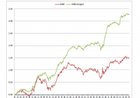
Long only, ETF investing, portfolio strategy, momentum “}); $$(‘#article_top_info .info_content div’)[0].insert({bottom: $(‘mover’)}); } $(‘article_top_info’).addClassName(test_version); } SeekingAlpha.Initializer.onDOMLoad(function(){ setEvents();}); How to enhancing a Buy and Hold strategy with Dual Momentum Model. Reduce volatility and portfolio draw-down with an ETF cutoff model. How to apply both absolute and relative momentum to portfolio management. How to triple portfolio returns over a stock-bond index fund. Beginning with the ten (10) ETFs identified in Mebane T. Faber and Eric W. Richardson’s book, The Ivy Portfolio , the following analysis shows how the IVY portfolio would have performed from June 30, 2006 through 6/11/2015 when a momentum model is applied to these ETFs. The ETFs using in this analysis are the IVY 10 plus SHY , our cutoff or “circuit breaker” ETF. Here is the portfolio strategy used with the IVY 10. Rank the ETFs as shown in the following table. Review period is every 33 days. This moves the review or update throughout the month, thus avoiding short-term trading fees, wash rule, and end of month mutual fund window dressing. Look-back periods are 87 days with a 30% weight, 145 days with a 50% weight, and 20% assigned to a 14-day mean-variance volatility setting. ETFs performing below SHY using this ranking system are sold out of the portfolio. Select the top two performing ETFs and invest equal percentages in each. If there is a tie, invest in equal amounts in the three or four top performing ETFs. The absolute momentum model identifies ETFs that are ranked above SHY. The ranking model identifies the relative momentum between the various ETFs. IVY 10 ETF Rankings: The following table (generated from spreadsheet) shows both the absolute and relative momentum for the 10 IVY ETFs. The following table includes 6/11/2015 data. GSG and VB are the top two performing ETFs based on the three metrics used to come up with these rankings. If one were to follow this model today, we would invest equal dollars in GSG and VB. (click to enlarge) IVY 10 Back-Test Results: How has this investing model worked since June 2006? The following graph shows a Monte Carlo calculation where the dark black line is the average performance of the IVY 10. The red line is the performance of our stock-bond benchmark, VTTVX . Note the light gray lines as they show other probabilities or noise around the review days. In reality, investors are likely to make trades from 2 days before the review period to as many as 5 days after the review period. Call this trading noise. Even the worst light gray line outperforms the VTTVX benchmark. Here are a few salient points when Dual Momentum is applied to the IVY or Faber 10. Portfolio return = 240% vs. 77% for the VTTVX index fund. Maximum draw-down (DD) for portfolio is 27% vs. 45% for VTTVX. Average annual DD for portfolio is 14% or under 15%, what might be considered an acceptable level. Average Compound Annual Growth Rate (CAGR) = 14.7%. Trades per review period = 1.7. Tax considerations may dictate one use this model only with tax-deferred accounts. (click to enlarge) Disclaimer: After running hundreds of back-tests using similar models to what is described above, there is still a considerable amount of luck when it comes to the day in which a particular ETF is purchased. The “trading noise” analysis helps to temper this problem, but it is still there. Also, the above model does not account for remaining cash that is left lying around due to dividends and money not invested due to share rounding. Taxes are also an issue as mentioned above. Investors in the 28% tax bracket need to add something close to 2% annually to overcome the difference between short and long-term capital gain taxes. Each investor should take their own tax situation into consideration. Disclosure: The author is long VTI,VEA. (More…) The author wrote this article themselves, and it expresses their own opinions. The author is not receiving compensation for it (other than from Seeking Alpha). The author has no business relationship with any company whose stock is mentioned in this article. Additional disclosure: Back-testing analysis was run by interested investor. Share this article with a colleague

A Revelation For Small-Cap Investing Strategies

Suddenly, business as usual for small-cap investing is in need of a makeover, thanks to a new research paper (a landmark study for asset pricing) that revisits, reinterprets and ultimately revives the case for owning these shares – after controlling for quality, i.e., “junk”. Cliff Asness of AQR Capital Management and several co-authors have dissected the small-cap effect anew and discovered that there is a statistically robust small-cap premium across time after all, but only for companies that aren’t wallowing in financial trouble of one kind or another. The paper’s title says it all: ” Size Matters, If You Control Your Junk .” At the very least, the study will reframe the way the investment community thinks about small-cap investing, perhaps leading to a new generation of ETFs in this space with freshly devised benchmarks. Does that mean that the enigma of the small-cap premium has been solved? Let’s put it this way: suddenly, the topic looks a lot less cryptic. For those who haven’t been keeping up-to-date on the strange case of the on-again, off-again small-cap premium, a growing pool of research has raised doubts about this risk factor. Although there was much rejoicing in the years following the influential 1981 paper by Rolf Banz ( “The Relationship between Return and Market Value of Common Stocks” ) – the study that effectively launched the industry of small-cap investing – the pricing anomaly has fallen on hard times in recent years. As Asness et al. advise: Considering a long sample of U.S. stocks and a broad sample of global stocks, we confirm the common criticisms of the standard size factor: a weak historical record in the U.S. and even weaker record internationally makes the size effect marginally significant at best, long periods of poor performance, concentration in extreme, difficult to invest in microcap stocks, concentration of returns in January, absent for measures of size that do not rely on market prices, and subsumed by proxies for illiquidity. This is old news, of course. What’s new is the finding that “controlling for quality/junk reconciles many of the empirical irregularities associated with the size premium that have been documented in the literature and resurrects a larger and more robust size effect in the data.” In other words, the small-cap factor is alive and kicking, but it requires some tweaking in how we think about this slice of equities, namely, by focusing on comparatively “high-quality” firms. In summary, controlling for junk produces a robust size premium that is present in all time periods, with no reliably detectable differences across time from July 1957 to December 2012, in all months of the year, across all industries, across nearly two dozen international equity markets, and across five different measures of size not based on market prices. The critical issue is that small-caps generally are populated with a relatively high share of “junky” firms. Whereas large firms tend to be of higher quality – defined by, say, profits or earnings stability – there’s a wider spectrum of dodgy operations among smaller firms. That’s not surprising, but it does have major implications for how we think about expected return in this corner of the equity market. It’s puzzling that no one’s documented this previously, at least not as thoroughly and convincingly as Asness and company have. In any case, the results speak loud and clear: if you’re intent on carving out a dedicated allocation to the small-cap factor, you’re well advised to do so by focusing on relatively high-quality firms in this realm of the capitalization spectrum. Keep in mind, too, that the findings don’t conflict with the value factor, although here too there may be a bit more clarity in the wake of the paper. In fact, the authors “find that accounting for junk explains why small growth stocks underperform and small value stocks outperform the Fama and French (1993, 2014) models.” Ultimately, the numbers speak volumes. The new paper slices and dices the data from several perspectives, and it’s worth the time to read through the details to understand how this study revises our understanding of small-cap investing. “Overall, there is a weak size effect, whose variation over time and across seasons is substantial, as documented in the literature,” the researchers write. The smoking gun is that the case for small-caps looks much stronger when sidestepping the junkiest firms. A graph from the paper summarizes the point. Indeed, the difference between the cumulative investment return for the conventional definition of small-cap (SMB, or small minus big) vs. the proxy defined by Asness et al. (SMB-Hedged) is quite stark over the past half century. (click to enlarge) The paper’s discovery amounts to an important revelation for asset pricing, and arguably something more substantial for investors who toil in the small-cap waters. In short, it seems that small-cap strategies, as currently designed, are in need of revising, perhaps dramatically so, depending on the portfolio, ETF or mutual fund. Yes, Virginia, there is a small-cap premium, but to harvest it in a meaningful way, we’ll have to rethink how we invest in these companies.