Tag Archives: function

Does The Presidential Cycle Have A Significant Impact On Stock Market Performance?

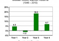
Summary The third year of a presidential cycle has historically offered outsized returns. In this study, data for 1928 to 2014 were analyzed to evaluate the effect of the presidential cycle on S&P 500 performance. Given that we are currently in Obama’s third year (of his second term), should we be expecting significant gains ahead? Introduction In a previous article entitled ” The January Effect Revisited And A Call For The Use Of Elementary Statistics “, I made the case that assertions of outperformance should be supported by elementary statistics. In the case of the January effect, I analyzed monthly data from 1988 to 2014 to show that the standard deviation of monthly returns was actually very large compared to the average return for any given month, rendering most of the observed seasonal deviations to be statistically insignificant. Yet, the absence of error bars on the most popular graphs illustrating the January effect means that investors studying the chart would be unable to ascertain whether [i] the outperformance is statistically significant and [ii] whether or not the increased return is worth the risk. The article ended with an exhortation for all analysts to incorporate simple statistical analysis into their charts. In the present article, we analyze another phenomenon that may be playing out at the present time: the impact of the presidential cycle (also known as the election cycle) on stock market performance. The following charts are top hits in a Google search for “presidential cycle stock market”. (Source: GoBankingRates ) (Source: Murray Financial Group ) (Source: Seeking Alpha ) (Source: John Rothe ) All four charts show the 3rd year of a president’s term to be the best in terms of stock market performance, and the 2nd year to be the worst. Interestingly, the last chart seems to show that the final quarter of the 2nd year actually delivers the best performance out of all 16 quarters in the presidential cycle. Now, what are all four charts missing? If you had read the previous article (or the introduction) you would know that the answer is “error bars”. Given that we are currently in the 3rd, and presumably “best”, year of Obama’s presidency (the second term), I was interested to determine whether or not the presidential cycle has a statistically significant impact on stock market performance. Results and discussion Yearly total return performance for S&P 500 (NYSEARCA: SPY ) from 1928 to 2014 was obtained from Aswath Damodaran . For the purposes of this study, the four-year presidential cycle is assumed to occur continuously even though there have been interruptions with certain presidents. For example, Gerald Ford’s first year in the office in 1974 would still be counted as the second year of the presidential cycle (since it would have been Richard Nixon’s 6th year in office). The S&P 500 annual total return distribution from 1928 to 2014 shows a bell-like shaped curve with a negative skew, from which the dreaded “left tail” can be observed. Yet, it should be noted that 63 out of the 87 years (or 72.4%) in this study have had positive returns. The average return over the 87 years was 11.53%, while the median return was 14.22%. This is one reason why “buy-and-hold” has worked so well for the average investor in the U.S. market. First let’s have a look at the average performance of the stock market over the four-year presidential cycle. (click to enlarge) Consistent with the charts presented in the introduction, we find that the 3rd year of the presidential cycle provides the greatest performance, with an average performance of 17.57% (and median of 22.34%). Moreover, the 3rd year was the only year that outperformed the average overall return of 11.53% (and median of 14.22%). The other three years all underperformed the average, with the 2nd year having the lowest return of 8.80% (and median of 10.00%), again consistent with previous charts. The next chart shows the data for average returns but with the inclusion of error bars representing the standard deviation of the results. (click to enlarge) We see that the standard deviation of the annual returns is larger than the actual returns (though not overwhelmingly so), indicating significant variability in the results. One way to visualize these error bars is to assume that about 68% (or just over two-thirds) of the data points lie between the error bars. A t-test was conducted to investigate whether or not the annual returns of each year of the presidential cycle is significantly different from the overall average return of 11.53%. The results are shown in the table below. 1st 2nd 3rd 4th Mean 8.99% 8.80% 17.57% 11.03% Standard deviation 22.01% 21.21% 18.90% 17.20% p-value 0.594 0.553 0.158 0.893 Significant? No No No No The results of the t-test show that none of the years of the presidential cycle are significantly different from the average year. A number of commenters in the previous article mentioned that because the return distribution is not exactly normal (there is some skewness or kurtosis), an alternative test such as the Wilcoxon test should be performed. Therefore, I also calculated the p-value using the one-sample Wilcoxon signed-rank test to determine whether the median returns for each year of the presidential cycle was significantly different from the overall median return of 14.22%. 1st 2nd 3rd 4th Median 7.40% 10.00% 22.34% 13.35% p-value p> 0.10 p> 0.10 p> 0.10 p> 0.10 Significant? No No No No Similarly, the one-sample Wilcoxon signed-ranked test shows that none of the observed performances were significant. (It is noted that the Wilcoxon test assumes a symmetrical distribution, which is not perfectly valid for the present distribution. I considered the one-sample sign test, but that test does not capture the magnitude of differences from the median. If anyone knows another simple one-sample, non-normal, non-symmetric test that can be used instead, please let me and the readers know!) C onclusion While the 3rd year of a presidential term has delivered, on average, outsized returns for the past 87 years (from 1928 to 2014), any deviations between any of the years of the presidential cycle and the average or median return were found to be insignificant. Note that statistical tests such as these do not “disprove” the presidential cycle effect, nor do they prevent you from profiting (or attempting to profit) from the perceived opportunity. What the tests do tell you is that for the past 87 years, any impact that the presidential cycle has had on stock market returns is indistinguishable from chance. Therefore, this article ends with another call for analysts to incorporate simple statistical analysis into their presentations. This information would allow investors to evaluate [i] whether the outperformance is statistically significant and [ii] whether or not the increased return is worth the risk. Author’s note: On a personal level, I was rather disappointed in the outcome of this study. Given that we are currently in the 3rd year of the presidential cycle, I was really hoping that the effect would be significant. I guess that’s confirmation bias creeping in!

S&P 500 FCF Analysis: What You Do Depends On Who You Are

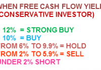
Analysis of the S&P 500 Index and its individual components using the “Free Cash Flow Yield” ratio. Specifically written to assist those Seeking Alpha readers who are using my free cash flow system. Generates a final result for the S&P 500 Index and explains that result to each reader depending an what type of investor they are. Back in December of last year, I introduced my free cash flow system here on Seeking Alpha, through a series of articles that you can view by going to my SA profile . My purpose in doing so was to try and teach as many investors as I could, on how to do this simple analysis on their own, as I believe in the following: “Give a person a fish and you feed them for a day, Teach a person to fish and you feed them for life” I have been very pleased with the positive feedback that I have received so far, but included in that feedback were many requests by those using my system, to see if they did their analysis correctly or not. Since the rate of these requests has been increasing with every new article I write, I have decided to start a new series of articles here on Seeking Alpha analyzing the S&P 500 Index, where I will analyze each of its components individually. That way those of you using my system will have something like a “teacher’s edition” that will give you all the correct calculations for each component. Obviously I can’t include the results for all my ratios in one article, so I will thus be doing a series of articles, where each ratio’s results for the S&P 500 Index will have its own article devoted to it. Hopefully these articles can be used as reference guides that everyone can use over and over again, whenever the need arises. Having said that, at the same time we will be “killing two birds with one stone” as we will also be analyzing the S&P 500 Index and give one final result for it as well as its individual components . That way these series of articles will also be able to give us a real time analysis of whether the S&P 500 Index is attractively priced or overvalued. In order to save space in this article (as the table that will soon follow is quite long) I would welcome everyone to read my article on how to analyze a portfolio/Index by clicking on the following link first: Warren Buffet s Berkshire Hathaway Portfolio: A Free Cash Flow Analysis That way those of you who are new to this analysis will get a complete introduction and for others already familiar with my work, let it act as a refresher course. This article with concentrate on my “Free Cash Flow Yield Ratio” Free Cash Flow Yield = Free Cash Flow per Share / Stock Market Price One key point to always remember in using this system, is that it is designed for all kinds of investors, whether you would be conservative (like I am) or a more aggressive/buy & hold investor. I have created the following parameters for each type and they are as follows: Finally it is also important to understand that I personally do not invest in financial firms as a rule, because it is quite difficult to get a very accurate free cash flow result. This is so because financial firms generate very little in the way of capital expenditures, thus the results you find below are basically just cash flow from operations. I still analyze them as they are part of the S&P 500 Index, but again I don’t invest in them as I find financial firms too complicated to analyze. This belief of not investing in financials, saved me from suffering the huge losses that this sector suffered in 2008-2009, which cost investors dearly. For those who disagree we can start a discussion on the matter in the comment section below, which will allow me to further elaborate on the matter. So without further ado here is my “Free Cash Flow Yield Analysis of the S&P 500 Index (NYSEARCA: SPY ) and its components: (click to enlarge) The final free cash flow yield result of 5.11% for the S&P 500 Index would be classified as a ” Strong Hold” for the more aggressive/ buy & hold investor and a “Weak Sell” for the more conservative investor, using the parameter tables I included at the beginning of the article . The weightings that you see in the index were generated by mirroring those used in the SPDR S&P 500 ETF . Also remember that the results shown above are just for one ratio and that this is not investment advice, but just the results of the ratio. The system outlined in this article and all that will follow, as part of this series, are just meant to be used as reference material to be included as just “one” part of everyone’s own due diligence. So in other words, don’t make investment decisions based on just this one result, but incorporate it as one part of your own due diligence.

Utilities And Other Industries: Capital Expenditures Vs. Depreciation

It is very common among new investors to assume that depreciation equals the capital expenditures required to keep the company in place. Free cash flow is usually calculated by subtracting the full value of the capital expenditures. This can be wildly inaccurate. The utilities industry has capital expenditures and depreciation that are very different. If all capital expenditures by utilities were maintenance, the industry would be bankrupt very quickly. It is important to understand what, where, how, and why the company you are researching is spending money on capital expenditures in order to value it. Capital expenditures (capex) include a wide variety of things companies spend money on. Capex can include buying land, fixing machinery, building a new plant, upgrading the power system, or many other items. Some of these items are to reduce expenses, increase production, or improve the production process. These are called growth capital expenditures because they improve the company above its performance prior to spending them. Other capital expenditures that keep the company at its current steady state are called maintenance capital expenditures. Most companies spend some capex in both the growth and maintenance bucket so it is important to determine how much of each in order to value the company. One of the industries where this is glaringly obvious is the utility industry. Utilities routinely spend lots of money to support new infrastructure as growth capex. They also spend money on maintenance capital expenditures to ensure their existing operations are in good shape and highly reliable. A high level summary of net income, depreciation, and capital expenditures for some of the major utility companies is shown in the following table. Utility Company 2013 Net Income (millions) 2013 Depreciation (millions) 2013 Capex (millions) Capex minus Depreciation (millions) Capex divided by Depreciation Dominion Resources (NYSE: D ) 1,697 1,390 4,104 2,714 2.95x NextEra Energy (NYSE: NEE ) 1,908 2,163 3,228 1,065 1.49x Duke Energy (NYSE: DUK ) 2,665 3,229 5,526 2,297 1.71x Exelon Corp (NYSE: EXC ) 1,719 3,779 5,395 1,616 1.43x Southern Company (NYSE: SO ) 1,644 2,298 5,463 3,165 2.38x As you can see from the table, the capital expenditures of the utility companies exceeds the depreciation charge, typically by several billion dollars for companies this size. If all of these capital expenditures were maintenance capital expenditures, the market would have to be completely insane to assign the earnings multiples shown in the following table. Utility Company Current Price/2013 Earnings Dominion Resources 25x NextEra Energy 27x Duke Energy 23x Exelon Corp 19x Southern Company 28x Average 24x Earnings multiples this high are usually reserved for high growth companies. Many of the new projects these utility companies are investing in will earn a regulated rate of return between 8% and 12% which doesn’t sound like a high growth company. If anything, this is close to an average company’s rate of return and generally average companies trade closer to 15x earnings. Depreciation is a noncash expense that reduces the net income reported. When valuing companies, it is generally advisable to add back depreciation to net income and then subtract maintenance capital expenditures to get a truer view of profit. In the case of utility companies, they generally spend less money on maintenance capital expenditures than they expense on their income statement as depreciation. This deflates their net income number which makes their price/earnings ratios look higher. The following table shows the capex numbers in relation to the net income numbers for the utility companies. Utility Company 2013 Net Income (millions) 2013 Capex (millions) Capex divided by Net Income Dominion Resources 1,697 4,104 2.42x NextEra Energy 1,908 3,228 1.69x Duke Energy 2,665 5,526 2.07x Exelon Corp 1,719 5,395 3.14x Southern Company 1,710 5,463 3.19x By looking at the capex divided by net income column it is very obvious that most of the capex must be growth capex. If most of the capex was maintenance capex and the cost of maintenance was 1.69x to 3.19x the amount of profit each company was making, they would be out of business very quickly. In addition, one of the quirks about the utility industry is that lots of its “maintenance capex” still plays into the regulatory assets that allow future rates to be raised to earn the cost of investment plus a predetermined return on equity. An easier way to track maintenance capex for utility companies is to read their filings and see how much and when the regulatory bodies approve expenditures to be counted towards the regulated rate of return. However, for companies that aren’t in the regulated utility industry, it can be more difficult to determine much of capex was maintenance capex. In general, it is a good idea to use the laws of large numbers when determining maintenance capex for companies that don’t specifically break it out. For example there could be two oil companies. Company A spent an average of $30 million on capex for each of the last few years and kept production flat. Company B spent an average of $30 million on capex for each of the last few years and production grew by 40%. Therefore it stands to reason that Company B was likely spending a much higher percentage of their capex on growth. Some companies half break it out by giving you a list of the major items they spent capex on and you can place each in the growth or maintenance bucket depending on the type. Maintenance capex should generally be determined over several years because things don’t break at the same frequency every year. This is more important for valuing small companies because larger companies generally spend similar amounts of maintenance capex every year. Another common capex that seems to be often included as an expense to reduce a company’s profit is when they buy or construct a new building for their corporate headquarters. This is actually growth capex because it will reduce future rent expense by the company (i.e. increase their profit) and it will appreciate over time. These are the reasons and some advice about making sure to understand the company’s capital expenditures when trying to value a company. It is especially important in the utility industry but even in other industries your valuations could be dramatically off without understanding where and why the company is spending money.