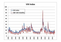
Summary Generally, it is far better to be a seller of equity market volatility than a buyer. VXX has returned -60% per year since inception. Negative roll yield has been the main culprit. Fortunately, expected roll yield can be objectively calculated every day – it is known ahead of time. Changes in the VIX Index are not knowable ahead of time, but can be partially forecasted using mean-reversion factors. A VXX forecasting model using roll yield and two VIX Index forecasting factors had a correlation with VXX of 54% since inception. When combined with a long position in the S&P 500, this “3-Factor VXX Strategy” boosted the S&P 500 portfolio return by 12.0% per year. The VIX Index and VIX Futures The Chicago Board Options Exchange [CBOE] Volatility Index, commonly referred to as the VIX Index, is an indication of volatility expectations for the S&P 500 over the next 30 days. It is based on the implied volatility of S&P 500 options traded on the CBOE. The graph below shows the history of the VIX Index since 1990, along with actual trailing 30-day volatility for the S&P 500. The VIX Index is closely associated with trailing monthly S&P 500 volatility, but tends to be somewhat higher than both trailing and coincident volatility most of the time. This upward bias in the VIX Index relative to actual realized volatility reflects the fact that investors are generally willing to pay a premium for the leverage provided by options. It may also reflect a demand for the kind of equity market “insurance” provided by S&P 500 put options and by long positions in VIX futures contracts. The VIX Index is not directly investable, but futures contracts based upon the VIX Index are investable. (click to enlarge) VIX futures contracts reflect expectations for the future price of the VIX Index, and as such, also reflect expectations for future S&P 500 volatility. VIX futures contracts are available for all twelve months of the year, and settle on either the third or fourth Wednesday of the month. VIX futures contracts settle based upon the value of the VIX Index on settlement date, so over time VIX futures contracts converge towards the level of the VIX Index, often referred to as the “spot price.” VIX-Related ETPs Many investors do not wish to trade in futures because of their unfamiliarity and perceived risk. At least nine VIX-related exchange-traded products (ETPs) are available that make investing in VIX futures easy. These VIX-related ETPs are tied to one of two indexes: The S&P 500 VIX Short-Term Futures Index, which allocates between the first and second VIX futures contracts to result in a constant weighted average maturity of one month. The S&P 500 VIX Mid-Term Futures Index, which allocates among the fourth, fifth, sixth, and seventh futures VIX futures contracts. Some VIX-related ETPs are exchange-traded funds (ETFs) that actually own portfolios of futures contracts, swaps, and short-term collateral. Others are exchange-traded notes (ETNs) that do not own actual portfolios, but instead are debt obligations of the issuers, usually large international banks. As such, they entail credit risk. The advantages of the ETNs, however, are that they may qualify for long-term capital gain treatment if held for more than a year and that they report their taxable income using Form 1099. The ETFs “pass-through” the 60/40 long-term/short-term tax treatment generally applicable to futures contracts. Also, the tax form they use is the Form K-1 rather than the more familiar Form 1099. Most investors dislike having to deal with K-1s. iPath S&P 500 VIX Short-Term Futures ETN (NYSEARCA: VXX ) By far, the largest and most liquid of the various VIX-related ETPs is the iPath S&P 500 VIX Short-Term Futures ETN. Most of the rest of this article will focus on VXX, but much of the analysis would apply to all VIX-related ETPs. As an ETN, VXX is an unsecured debt obligation of Barclays Capital, the issuer. Barclays pays the holder a return based upon the S&P 500 Short-Term VIX Futures Index, which offers exposure to a daily rolling long position in the first and second month VIX futures contracts designed to provide a constant one-month average maturity. Investors pay Barclays an expense ratio of .89% for this ETN. Most investors use VXX as a hedge against U.S. equity market exposure. Depending upon the time period and calculation methodology, VXX has a beta relative to the S&P 500 of roughly between -3.00 and -5.00. For example, at its average beta of around -4.00, VXX would be expected to increase by 40% if the S&P 500 declined by 10%. That is a lot of negative beta leverage, which is an attractive feature for many investors. However, owning VXX has been an expensive form of market insurance much of the time. The graph below shows the steady downward march of the historical return of VXX since its 1/29/2009 inception. Its compound annual return has been -60.38%. Periods of positive return have been infrequent and short-lived. The graph uses a log scale so that the slope of the line has the same meaning throughout the return history. To give some perspective on what a cumulative log return of -586% means: an unfortunate investor who bought $1,000,000 worth of VXX at its initial offering would, as of May 31, 2015, have only $2,842 left. (click to enlarge) The Three Components of VXX Return The S&P 500 VIX Short-Term Futures Index, upon which VXX is based, is affected by three factors: Roll yield Changes in the VIX futures term structure Interest on futures collateral Historically, most of the return from investing in the futures markets has come from roll yield rather than changes in the spot price. Roll yield (explained below) is particularly important in the VIX futures market. A change in the “spot” VIX index (the underlying index for VIX futures contracts) will affect all VIX futures contracts, though to varying degrees. Typically, the VIX futures contracts nearest to expiration will be affected the most, but sometimes the VIX futures term structure will change independently of changes in the spot VIX index. Since futures contracts do not require much margin, most of the cash is invested in various types of low-risk “collateral” investments, such as short-term Treasury bills. In recent years, interest rates have been so low that interest on futures collateral has not added much to return. Roll Yield The blue line in the graph below depicts the average month-end prices for the VIX index (spot) and for the first four generic VIX futures contracts (G1, G2, G3 and G4) since the 1/29/2009 inception of VXX. G1 is the “nearby” or generic futures contract expiring next – somewhere between 12 and 21 days after month-end. The nearby (G1) contract will ultimately be closed and settled for cash based upon the VIX index on settlement date. When the nearby contract is higher than the spot price, the market is said to be in “contango.” The opposite condition, when the nearby is lower than the spot price, is called “backwardation.” On average, the VIX futures market has been in contango – the blue line slopes upward. “Roll yield” refers to the fact that, unless the pricing structure for VIX spot and futures contracts changes, the price of the nearby (G1) contract will “roll” down to the spot price at settlement. Likewise, the price of the G2 will roll down to the G1 price, and so on. Since VIX futures trade each month, contracts are roughly 30 days apart (though the actual number of days between contracts varies between 27 and 35). The large negative roll yield of the G1 and G2 VIX futures contracts that comprise the S&P 500 VIX Short-Term Futures Index explains most of the negative return of VXX. (click to enlarge) Calculating the roll yield any point in time is a fairly straightforward, if tedious, process. Take for example the VIX futures term structure on 5/31/2015, depicted in the red line in the graph above. Here are the relevant inputs: (click to enlarge) The nearby G1 contract will roll down from 14.625 to 13.84, a roll yield of -5.37%. This will happen over just 17 days. That’s a daily roll yield of -.32%. The G2 contract will roll down from 15.825 to 14.625 for a roll yield of -7.58%, which will happen over the 35 days between the expiration of G1 and G2 for a daily roll yield of -.22%. VXX always has some combination of these two exposures (G1 and G2) that sum to 100%. The percentage allocations are provided each day on the “Index Components” page of the Barclays iPath ETN website for VXX . If we assume a constant 30-day maturity, then 17/30, or 57%, was allocated to G1, leaving 43% allocated to G2. Thus the weighted average daily roll yield on 5/31/2015 was -.27%, which annualizes to roughly -97%! That’s a lot to pay for equity market insurance! Disaggregating VXX’s Historical Return The graph below depicts a disaggregation of the VXX return since inception. Once the total VXX return (blue line) is adjusted for roll yield, the remaining return (red line) becomes much less negative, though the volatility of the two return series remains roughly the same at about 16%. This makes intuitive sense. Roll yield is a more-or-less constant daily drag on performance that cumulates steadily over time. But short-term performance shocks are mostly explained by changes in the level of the VIX index. Once this factor has been subtracted out, the remaining return series (green line) becomes flatter, with about half the volatility (a standard deviation of around 8% vs. 16%). (click to enlarge) Changes in the VIX Futures Term Structure In the graph above, the difference between the red line and the green line reflects the adjustment for changes in the spot VIX Index. Changes in the spot level explain much of the changes in the full VIX futures term structure, but not entirely, since not all shifts in the VIX futures term structure are parallel. If they were, the green line in the graph above would reflect only interest on futures collateral and it would be nearly flat. The graph below depicts term structures in VIX futures contracts since 12/31/2005, which is as far back as good data is available on Bloomberg. These historical month-end prices have been sorted from highest spot price to lowest spot price, and grouped by decile and quintile. Note how the spot VIX tends to move like the end of a whip, with more extreme moves than further out the term structure, which is more stable. These non-parallel shifts are why changes in the spot VIX do not fully capture all of the effects of changes in the VIX futures term structure. (click to enlarge) Interest on Futures Collateral Before 2008, interest on futures collateral was a significant component of return. Since then, however, interest rates have been so low that the impact of this category has been negligible, as shown in the graph below. Since the 1/29/2009 inception of VXX, its entire history has been during the ultra-low interest rate environment. (click to enlarge) Explaining VXX Return The exhibit below presents the results of a regression in which roll yield and change in spot VIX are used to explain the monthly return of VXX since inception. These two variables explain the vast majority of VXX return – 84%. Both are highly significant, with t-statistics of 10.28 and 18.69 respectively, and p-values (measuring the probability that the results are due to chance) well below 1%. The intercept rounds to zero, indicating that as mentioned above, the interest on futures collateral has been negligible. (click to enlarge) To be clear, we are calculating 30-day roll yield at month-end and using it to explain VXX return in the following month . We are using change in the VIX Index to explain VXX return in the same month . These two variables are somewhat negatively related to each other. Since 1/2009 (VXX inception), the correlation between the roll yield and change in VIX was -24%. It would have been more highly negative except for one outlier data point, as shown in the graph below: (click to enlarge) It makes intuitive sense that these two variables should have a negative relationship. The graph several graphs above showing historical VIX spot and futures contract prices sorted by spot price suggested a negative relationship. When spot VIX was at its lowest levels, the roll yield was at its most negative. In such circumstances, the market expected the VIX to increase in the months ahead, and this outlook was reflected in the futures prices. When spot VIX was at its highest levels, roll yield was positive and the futures prices forecast a decline in the VIX. Forecasting Changes in the VIX Index Our ultimate objective is to be able to forecast monthly VXX return so that we know when to invest in it, long or short. We already have one excellent variable for doing this – roll yield. It can be calculated accurately at the start of the month and provides an excellent forecast for VXX return over the course of the coming month. The regression above indicated a beta coefficient of 1.09 with a t-statistic of 10.28. Rarely are such good forecasting variables available in the world of investments. In the regression above, the change in VIX was calculated concurrent with monthly VXX return – that is, perfect foreknowledge of the change in VIX was assumed. The concurrent change in VIX was a highly significant variable in explaining VXX return, with beta coefficient of .73 and a t-statistic of 18.79. From the scatter graph above, we know that there is a negative relationship between roll yield and change in VIX, so it would be potentially dangerous to ignore either one. For example, if we use only roll yield in making our VXX forecasts, we are likely to invest long in VXX when the roll yield is the highest (most positive – when the market is in backwardation). Unfortunately, these times are also when the VIX Index is at its highest level, and (if there is any mean-reversion) these may be just the times when a change in the VIX is most likely to be negative. Despite an attractive positive roll yield, our long investment in VXX could easily provide a negative return (and possibly a large negative return) if the VIX moves down. In order to forecast monthly VXX return, it will be necessary to forecast monthly change in the VIX Index. Is there any way to forecast changes in the VIX over the next month? In fact, I have found two factors that are somewhat helpful. Both rely on the powerful statistical principal of central tendency: Mean reversion: reversion of the current VIX towards its exponentially-weighted 12-month moving average Expected-Actual: reversion of the current VIX towards its expected value given the current 30-day trailing volatility of the S&P 500 The historical pattern of equity market volatility spiking up and then falling back towards normal has been well documented by researchers. What is a “normal” level for the VIX? As shown in the graph below, since the 1/2009 inception of VXX, the VIX has been quite unstable. However, a reasonable measure of central tendency is the exponentially-weighted 12-month moving average. In my forecasting model, the further away the current VIX is from this mean, the greater the mean-reverting change in VIX forecast for the following month. (click to enlarge) As shown in the graph below, the trailing 30-day volatility of the S&P 500 Index has a statistically strong relationship with the current VIX level. I use a 120-month regression to forecast what the expected VIX level should be given trailing 30-day S&P 500 volatility. In a similar vein to the factor above, the further away the current VIX is from this expected level, the greater the mean-reverting change in VIX forecast for the following month. (click to enlarge) How do I translate these two factor concepts into actual forecasts of VIX change? This is where the art of model building comes in. My methodology involves a lot of rigorous statistical analysis that is well beyond the scope of this paper. Suffice it to say that honest quantitative researchers carefully avoid using any information that they would not have known at the time being tested, such as what “the best” methodology was going to be. Less honest (or less experienced) researchers often try various approaches and pick the one that renders up the strongest historical results. Often this “back-fitting” or “data-mining” procedure results in future “live” performance that is far weaker than indicated in the back test. I don’t do that. I have a well-developed set of statistical techniques that I use for a given statistical circumstance. I have used them for many years. They not only speed up my research since I don’t have to reinvent them every time, but they also keep me honest by avoiding trial-and-error iterations using various techniques. Using my usual statistical processes, I have derived forecasts in the change in the VIX over the following month based upon the two measures of central tendency described above. The regression results below measure the statistical power of those forecasts. It should not be surprising that this two-factor VIX model predicts only about 21% of the variability in the VIX since 1/2009. Many factors can affect the VIX, and most of them are unforecastable. On the other hand, both of the variables, labeled “Mean Reversion” and “Expected-Actual” in the regression table, are statistically significant at the 2% level (i.e., there is only a 2% probability that their predictive power is due to random chance). (click to enlarge) Forecasting VXX When this two-factor VIX forecasting model is combined with the roll yield calculations used above to forecast the return in VXX (the ETN), the model does a decent job of forecasting the fund’s return (though not nearly as good as the 84% explanatory power of the first regression above that assumed perfect foresight of the change in VIX). As shown below, this regression explains 30% of the VXX return. All three factors are highly significant, with t-statistics well above 2.0 and p-values (measuring the probability that the results are due to chance) of less than 1% in every case. (click to enlarge) Since all three factors are forecasts of percentage change in either the VIX Index or in VXX over the next month, they are all on roughly the same scale. Thus, a simple method for combining them into an overall forecast is simply to add them together. The resulting forecasts are depicted in the graph below. Note the preponderance of negative forecasts. This is primarily the result of the fact that roll yield is normally negative. (The average 30-day month-end VXX roll yield since its inception has been -6.85%). (click to enlarge) The correlation between this 3-factor forecast model and actual VXX return over the following month has been 55% since inception. (This is quite close to the regression output above that shows an “R” of 57% using the optimal weights on each of the three factors. In our portfolio simulation, by simply adding them together, we are giving them equal weights since we would not have known what the optimal weights were back in time). Any experienced quantitative researcher would say that a correlation of 55% is extremely high. It is certainly high enough to warrant using it in real portfolios. However, if a negative return forecast for VXX implies a negative portfolio position, then implementation will normally require a short position in VXX. (More below on why inverse VIX ETNs, such as XIV, may not be a very attractive substitute for a short VXX position). Fortunately, VXX is extremely liquid and easy to borrow. For example, my broker (Interactive Brokers) has well over 2 million shares available at an annual borrow cost of about 2.5%. VXX Portfolio Strategy Simulation Translating a forecast into a portfolio strategy involves a combination of experienced judgment and a set of statistical risk and return tradeoff calculations beyond the scope of this paper. However, a greatly simplified methodology can still prove illustrative. In the graph below, the VXX return forecast has been directly translated into a portfolio position. That is, a forecast of -10% was translated into a (short) portfolio position of -10%. Returns for the Strategy are shown in the blue line. The average position in VXX for the 3-Factor Strategy was -5.83%, so a plot of this buy-and-hold implementation (red line) was provided for comparison. Transaction costs of .10% on all trades were included (this is higher than the actual bid-ask spread) as well as borrow cost at a rate of 2.5%. (click to enlarge) During the 6+ years of the historical simulation, the compound annualized return of the 3-Factor VXX Strategy (blue line) would have contributed 10.5% to a portfolio with an average capital commitment of 5.83% (leaving 94.17% to be invested elsewhere on average). If that same 5.83% had been allocated to a short position in VXX at the beginning of each month, the return contribution would still have been a very respectable 4.1% per year (red line). The annualized risk/return ratio of the Strategy was about 1.8. As is typical of any strategy, and particularly one that uses a single security, there were periods of negative performance. The largest drawdown was 6.5%, ending on 12/31/2014. The Strategy experienced below-average performance in 2014, but so far in 2015, it has resumed its historical trajectory. Most importantly (and perhaps surprisingly), the 3-Factor VXX Strategy was virtually uncorrelated with the S&P 500. Its correlation with the S&P 500 was only 16%, with a beta of only .06. As shown below, the portfolio diversification benefits of combining the 3-Factor VXX Strategy with the S&P 500 boosted the compound annualized return from 17.1% to 29.1%, an increment of 12%. This is just the kind of alternative/uncorrelated return that investors are searching for to diversify the equity market risk in their portfolios. (click to enlarge) XIV: Caution on Inverse VIX ETPs The 3-Factor VXX Strategy described above called for being short VXX most of the time. But short selling is unfamiliar territory for many investors. They may perceive it as risky because of the risk of unlimited loss, even though shorting may have the effect of reducing the risk of an overall portfolio. Also, some investors, such as IRAs and tax-exempts, may be prohibited from selling short. These investors may be tempted to implement the VXX strategy using one of the inverse VIX ETPs. This section is intended to provide a note of caution for such investors. The VelocityShares Daily Inverse VIX Short-Term ETN (NASDAQ: XIV ) is by far the largest and most liquid of the inverse VIX ETPs, so I will focus on it. However, the conclusions drawn here are no doubt applicable to any daily reset inverse ETPs based on a short-term VIX index, of which there are several. The inception date of XIV was 11/29/2010. Its benchmark index is the same one as for VXX – the S&P 500 VIX Short-Term Futures Index. As an ETN, XIV is an unsecured debt obligation of Credit Suisse AG, the issuer. The note’s return is tied to the inverse performance of the underlying index on a daily basis less the 1.35% expense ratio. Because the hedge ratios used in XIV are reset daily, its returns will not be the same as a short position in VXX. The difference arises from something called “volatility drag” (or “volatility loss”). I have written much more extensively on this subject before, so I won’t go into an explanation here. Interested readers should take a look at my previous paper . As shown in the graph below, a short position in VXX has modestly outperformed a long position in XIV since XIV’s 11/29/2010 inception. (The comparison includes an assumed borrowing cost of 2.5% per year for VXX – the rate currently charged by Interactive Brokers). A difference of 2.4% per year may not seem like much, but there is considerable variability around this average. For example, in October of 2014, short VXX outperformed XIV by 10.89%, but in February of 2015, it underperformed by -6.27%. The standard deviation of monthly return difference was 4.32% since the inception of XIV. Volatility drag is “path dependent” in that the patter of daily returns matters a great deal. (click to enlarge) Volatility drag is particularly large for XIV because of its high volatility. As I mentioned in my earlier paper, volatility drag is positively related to the volatility of the underlying index (hence the term “volatility drag”). I have a statistical model that I use to forecast volatility drag over the next month for inverse ETFs. The average forecast of volatility drag for XIV in my model has been in the range of .5%-2% per month . That is high enough to make a short position in VXX more attractive than a long position in XIV, at least for those able to short. Although volatility drag may be mitigated to some extent by frequently rebalancing position sizes, this may be expensive and impractical for most investors. On top of that, even the daily returns of XIV have not matched the inverse of the returns of the S&P 500 VIX Short-Term Futures Index very well. Bloomberg has daily returns for XIV starting on 11/30/2011 (a year after inception), and since then, the average daily absolute difference between the fund return and the benchmark index return has been 0.82%. This is a very high level of “basis risk.” While the positive differences have largely offset the negative differences, the fund has fallen behind its benchmark by .02% per day on average, which annualizes to under-performance of about 5% per year. (Remember that the 2.4% difference between short VXX and long XIV cited above included a borrow cost of 2.5% per year for shorting VXX). Thus, even very short-term use of XIV will expose an investor to daily basis risk (the risk that you will happen to buy it right before a day when it falls far short of its benchmark index). As the expected holding period for XIV lengthens, basis risk becomes less of a concern, but volatility drag becomes more of a concern. Summary and Conclusion VXX is usually bought by investors hoping it will provide a hedge against equity market risk, but it has proven to be very expensive insurance, with an annualized return since its 1/29/2009 inception of -60.38%. The primary cause of the negative return has been negative “roll yield” as the nearby VIX futures contracts have on average been priced considerably higher than the spot VIX index towards which they will converge at settlement. VXX’s roll yield can be calculated at any time, and provides a very powerful forecast for VXX return over the following month. The other important component of VXX monthly return is the change in the VIX index that takes place during the month. Unlike the roll yield, this component cannot be known ahead of time. However, the VIX index does exhibit strong mean-reversion. Two measures of central tendency, 1) 12-month exponentially-weighted moving average of VIX and 2) expected VIX based on trailing 30-day S&P 500 volatility, have proven statistically powerful in forecasting change in VIX over the coming month. These two VIX change forecasting factors plus the month-end roll yield combine to provide a good forecast for VXX return in the coming month, explaining 30% of VXX returns. VXX return forecasts were negative most of the time since the fund’s inception, calling for short positions in VXX. A simple one-for-one translation of these forecasts into VXX portfolio positions was tested. For example, a forecast of -10% meant a -10% (short) position in VXX. This 3-Factor VXX Strategy provided a compound return since inception of 10.5%, with a correlation to the S&P 500 of only 16%. The 3-Factor VXX Strategy, when combined with a long position in the S&P 500, achieved a compound average return of 29.1% since inception, an increment of 12.0% over the 17.1% return of the S&P 500 itself. This illustrates the power of portfolio diversification. Such a characteristic is exactly what is sought by most investors who purchase (usually ill-advised) long positions in VXX, when normally they should be selling it short. Unfortunately, a long position in an inverse VIX ETP is not equivalent to a short position in VXX. The largest and most liquid of these, XIV, has underperformed a short position in VXX by an average of 2.4% per year since the 11/29/2010 inception of XIV. Most of its performance shortfall is due to “volatility drag.” XIV also has experienced large daily deviations from its benchmark index, a phenomenon known as “basis risk.” These two considerations make it a less attractive investment than shorting VXX. Bottom line: Short VXX when the roll yield is attractively negative unless the VIX index is unusually low, but don’t buy XIV as a substitute unless you can’t short. Disclosure: I am/we are short VXZ IN LONG/SHORT PORTFOLIOS AND LONG ZIV IN LONG-ONLY PORTFOLIOS. (More…) I wrote this article myself, and it expresses my own opinions. I am not receiving compensation for it. I have no business relationship with any company whose stock is mentioned in this article. Additional disclosure: My long and short positions change frequently, so I make no assurances about my future positions, long or short. The information contained in this article has been prepared with reasonable care using sources that are assumed to be reliable, but I make no representation or warranty regarding accuracy. This article is provided for informational purposes only and is not intended to constitute legal, tax, securities, or investment advice. You should discuss your individual legal, tax, and investment situation with professional advisors.