Scalper1 News
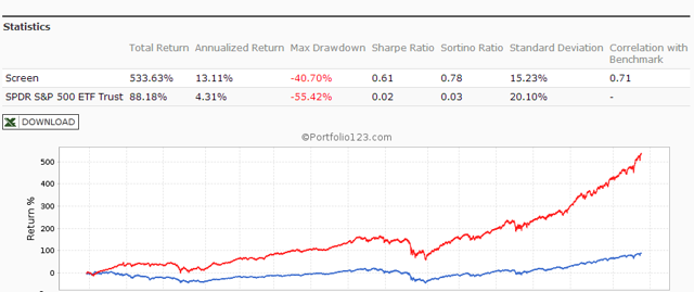
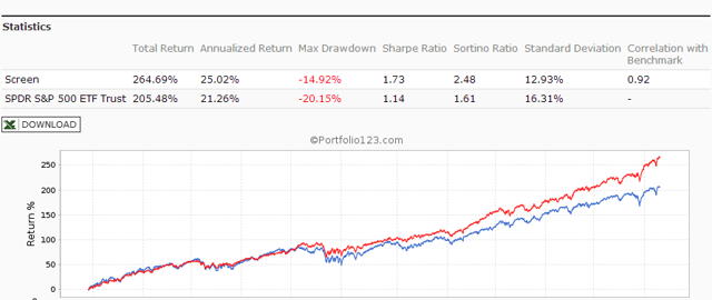
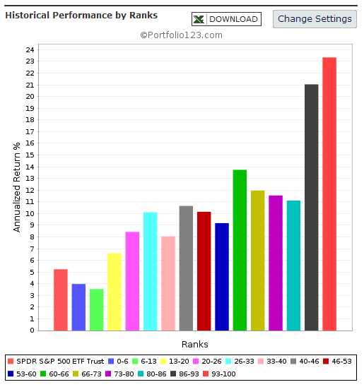
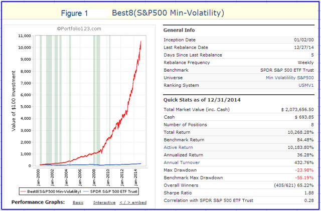
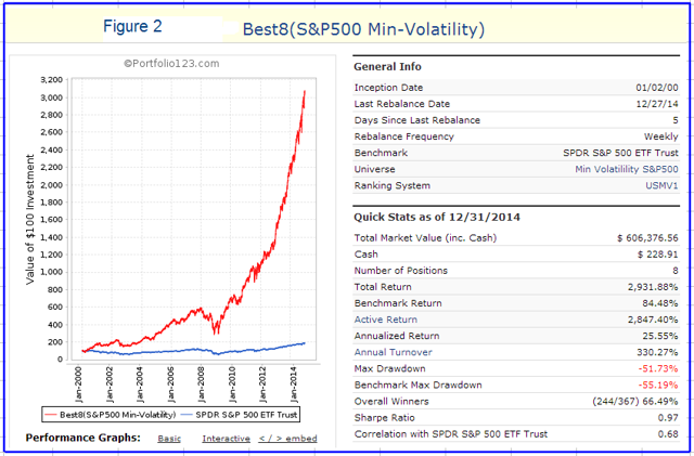
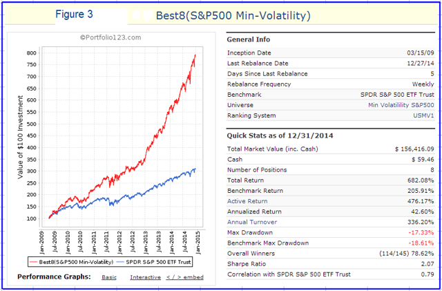
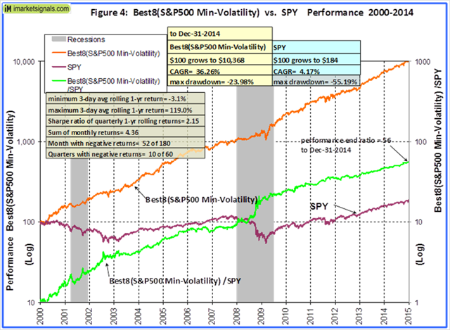
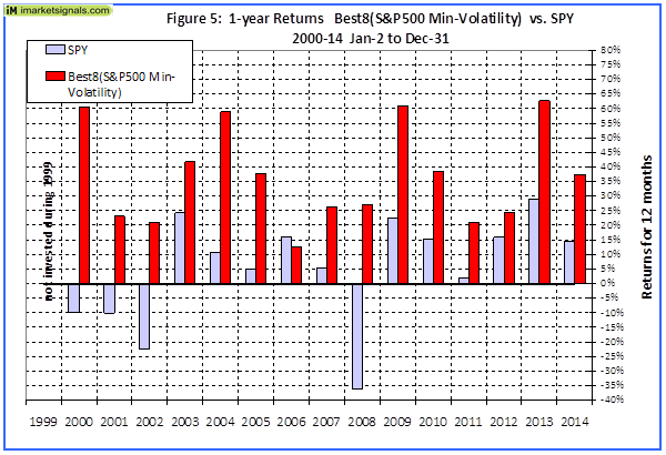
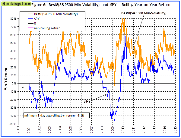
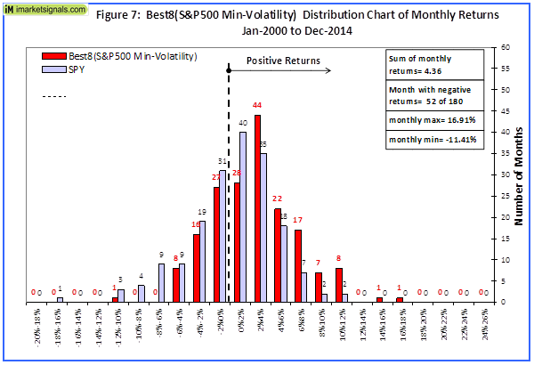
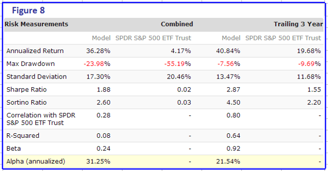 Originally published on Jan. 2, 2015 This R2G model trades in highly liquid large-cap stocks selected from those considered to be minimum volatility stocks of the S&P 500 Index. When adverse stock market conditions exist the model reduces the size of the stock holdings by 60% and buys the -1x leveraged ProShares Short S&P500 ETF (NYSEARCA: SH ). It produced a simulated survivorship bias free average annual return of about 36% from Jan-2000 to end of Dec-2014. Minimum volatility stocks should provide exposure to the stock market with potentially less risk, seeking to benefit from what is known as the low-volatility anomaly . Consequently, they should show reduced losses during declining markets, but should also show lower gains during rising markets. However, our backtests show that better returns than the broader market can be obtained under all market conditions by selecting 8 of the highest ranked stocks of a universe made up from minimum volatility stocks of the S&P 500. Minimum volatility stock universe of the S&P 500 By definition, minimum volatility stocks should exhibit lower drawdowns than the broader market and show reasonable returns over an extended period of time. It was found that a universe of stocks mainly from the Health Care, Consumer Staples and Utilities sectors satisfied those conditions. This minimum volatility universe of the S&P 500 currently holds 119 large-cap stocks (market cap ranging from $4- to $295-billion), and there were 111 stocks in the universe at the inception of the model, on Jan-2-2000. Performance of all the stocks in the universe from 2000 to 2014 The backtest period was 15 years, from January 2000 to December 2014. The backtest simulates holding all stocks of the universe equal weight and rebalancing every week to equal weight. Dividends are included in the stock price data, and are therefore accounted for in the backtest. The maximum drawdown during the backtest period would have been 40.7%, considerably less than the 55.4% for SPY , the SPDR S&P 500 ETF Trust. Annualized return (CAGR) of 13.1% was also considerably better than the 4.3% for SPY. (click to enlarge) (click to enlarge) Performance of all the stocks in the universe during up-market conditions The period March 2009 to December 2014 qualifies as an up-market period. The maximum drawdown would have been 14.9%, less than the 20.1% for SPY. The backtest shows an annualized return of 25.0%, marginally better than the 21.3% for SPY. (click to enlarge) (click to enlarge) The Best8(S&P500 Min-Volatility) model One can see from the above analysis that our S&P 500 minimum volatility stock universe provided better returns than what is expected from minimum volatility ETFs, showing less drawdown during declining markets, but also exhibiting gains during rising markets, similar to, or better than, the broader market. Therefore this universe provides the basis for periodically selecting the highest ranked 8 stocks according to a ranking system. Ranking System To find stocks which may be undervalued, all stocks of the S&P 500 point-in-time minimum volatility stock universe were ranked weekly according to the following parameters: Valuation (measured as market capitalization, debt and cash relative to earnings before interest, taxes, depreciation & amortization, future cash flow and projected earnings), Efficiency (measured as future cash flow relative to total assets), Financial Strength (measured as future cash flow relative to total debt), Short Interest (being the short interest ratio), Trend (measured as the stock price relative to a moving average of the price), with the highest rank obtainable being 100. To test the effectiveness of the ranking system, the universe was divided into 15 “buckets”, each holding about 8 stocks and performance was tested over 15 years. One can see that the “bucket” on the very right with the highest ranks also shows the highest annualized return of about 23%. (Note, there are no buy- and sell-rules in the ranking system.) Trading Rules The model assumes stocks to be bought and sold at the next day’s closing price after a signal is generated. Variable slippage accounting for brokerage fees and transaction slippage were taken into account. (See the Appendix for variable slippage.) Taxes are assumed to be deferred, as for retirement accounts. Buy Rules: Short Interest Ratio < 2.8, and exclude some of the largest market cap stocks from being selected. Sell Rules: Performance In the figures below the red graph represents the model and the blue graph shows the performance of benchmark SPY. Figures 1, 2 and 3 show performance comparisons: Figure 1: Performance 2000-2014 and hedging with SH. The model reduces the size of the stock holdings by 60% to buy SH during down-market conditions. (Note: The inception date of SH was June 19, 2006. Prior to this date values are “synthetic”, derived from the S&P 500.) Annualized Return= 36.3%, Max Drawdown= -24.0%. Figure 2: Performance 2000-2014 without hedging. Annualized Return= 25.6%, Max Drawdown= -51.7%. Figure 3: Performance 2009-2014 without hedging. Annualized Return= 42.6%, Max Drawdown= -17.3%. (click to enlarge) (click to enlarge) (click to enlarge) (click to enlarge) (click to enlarge) (click to enlarge) Figures 4 to 8 show performance details: Figure 4: Performance 2000-2014 versus SPY. Over the 15-year period $100 invested at inception would have grown to $10,368, which is 56-times what the same investment in SPY would have produced. Figure 5: 1-year returns. Except for 2006 the 1-year returns were always higher than for SPY. There was never a negative return over one calendar year. Figure 6: 1-year rolling returns. The minimum 1-year rolling return of the 3-day moving average was -3.1% early in 2009. Figure 7: Distribution of monthly returns. One can see that the monthly returns follow a normal distribution, displaced to the right relative to the returns of SPY. Figure 8: Risk measurements for 15-year and trailing 3-year periods. (click to enlarge) (click to enlarge) (click to enlarge) (click to enlarge) Liquidity To calculate the maximum dollar-value of a portfolio without incurring too much slippage the following formula was provided by P123: ($LiquidityBottom20Pct * #Position * 5%) / WeeklyTurnover% where 5% is the maximum amount traded without affecting the stock price. $LiquidityBottom20Pct = $ 16.8-million #Positions = 8 Annual Turnover% = 430% WeeklyTurnover% = 8.3% Maximum Portfolio Size = ($16.8 * 8 * 5%) / 8.3% = $80-million Thus, this model could accommodate a good number of individual investors. Variable Slippage The model assumes that stocks are bought/sold at the next day’s closing price after the signal is generated. Since one may not be able to obtain the closing price, a slippage factor is applied to account for a possible higher/lower price for the transactions. The slippage percentage is calculated for every transaction based on this algorithm: 1) The 10 day average of the daily traded $-amount is calculated (price*volume). 2) The slippage is set according to where the average falls in this table: 0 – $50K 5.00% $50K – $100K 1.50% $100K – $350K 0.75% $350K – $1M 0.50% $1M – $5M 0.25% $5M+ 0.10% 3) Add (1/ Price)% to the result from Step 2. For example, Step 3 would add 1% to the slippage if the stock trades at $1, 0.1% if it trades at $10, etc. For the following transaction Date Symbol Type Shares Trading Volume on day Price excluding slippage 5/28/2013 XXX BUY 64,108 3,338,776 50.27 the slippage percentage would be (0.10 + 1/50.27) = 0.120% of $50.27, amounting to about 6 cents per share. So the average price per share paid for this transaction is $50.33. Scalper1 News
Scalper1 News