Scalper1 News
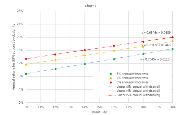
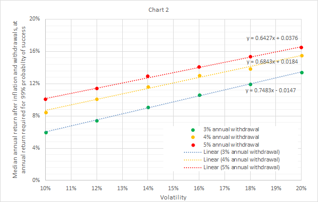
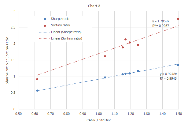
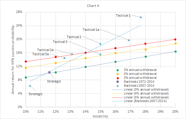
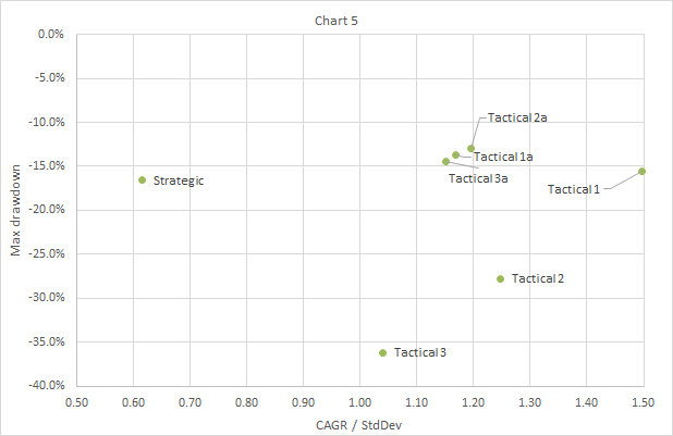
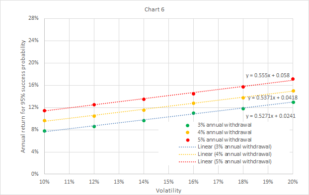
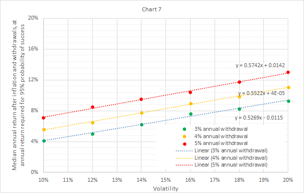 Summary A method is presented for evaluating risk of investment portfolios in retirement. This analysis defines risk as the chance of going broke during retirement, rather than a portfolio’s volatility. For adaptive asset allocation portfolios studied here, increasing volatility leads to decreasing risk. Introduction Investors benefit from availability of low-cost exchange-traded and mutual funds, and from myriad choices of strategies and tactics for allocating assets to a portfolio of these funds. Investors also have access to web-based tools to back test portfolio return and volatility. Then they can use those results as inputs to other web-based tools, to estimate worst-case and median future performance, taking into account planned contributions to the portfolio (for workers) or withdrawals (for retirees). What seems missing, however, is a systematic method to combine these tools to gauge the suitability of a portfolio for an investor’s own circumstances, and to reach a buying decision. For example, consider a recently-retired investor who needs to withdraw 3% of his or her savings per year, evaluating a choice between two portfolios: one with back test results showing 10% volatility and 9% annual return, and the other showing 18% volatility and 15% annual return. This analysis illustrates a method for making such a choice. The method has limitations, because back tests can turn out to be poor predictors of out-of-sample (future) performance, and because investors can feel uncomfortable using past performance as the only input to a decision — excluding other sources such as expert opinions on macroeconomic or political situations. However, the proposed method has the merit of providing an unemotional way to make an asset-allocation decision, based on easily-available data and tools. Consider a retired person who: Invests an initial amount at the start of retirement, Withdraws a percentage of the initial amount each year, adjusted for inflation, and Follows an asset class allocation strategy for the duration of retirement. Some advisors define a portfolio’s risk as its volatility, where volatility is an estimate of the standard deviation of annual returns. This is not helpful for choosing between portfolios when one has higher volatility and higher return than the other. A retiree could define risk less abstractly, as the chance of running out of money during retirement. A prudent retiree would first seek to reduce that risk to a negligible level, to avoid the catastrophe of going broke. That ensured, the retiree would next seek to increase the balance at the end of retirement, to leave a legacy. Simulation method This analysis used a Monte Carlo simulation tool at portfoliovisualizer.com , with input parameters set as shown in the table below. For each combination of annual withdrawal and volatility shown in the table, the analysis tried various values of expected return, until the simulation output showed a 99% probability of success. This means that at the preset annual withdrawal and volatility settings, 99% of Monte Carlo trials showed a positive balance at the end of retirement. In other words, the retiree did not go broke. The expected return setting that yields 99% probability of success represents the average annual rate of return necessary throughout retirement, to reduce risk to a negligible level at the given settings for annual withdrawal and volatility. Defining negligible risk as 99% probability of success (1% risk) seems appropriate considering the severity of the consequences of running out of money. The simulation tool also provides a median end balance, which gives the retiree’s legacy at the end of retirement in 50% of Monte Carlo trials at the given withdrawal rate and volatility settings, and at the expected return necessary for 99% probability of success at those settings. The simulator shows median end balance discounted for inflation, and therefore expressed in the same dollars as the initial invested amount at the start of retirement. Initial amount $1,000,000 (in today’s dollars) Annual adjustment Withdraw fixed amount annually Annual withdrawal $30,000, $40,000, or $50,000 for 3%, 4% or 5% annual withdrawal rate Inflation adjusted Yes Simulation period (years) 30 Simulation model Parameterized Returns Distribution Fat-Tailed Distribution (Student’s t-distribution with 30 degrees of freedom) Expected return Varied for combination of annual withdrawal setting above and volatility setting below, to obtain 99% “Probability of success” (1% risk of zero balance at end of retirement) Volatility Repeated at 10%, 12%, 14%, 16%, 18%, or 20% Inflation model Historical inflation (4.18% mean and 3.14% standard deviation, based on CPI-U from 1972 to 2014) This procedure yielded (volatility, return) pairs at 1% risk of going broke, for withdrawing an inflation-adjusted fixed amount annually, equal to 3%, 4%, or 5% of the initial amount. It also provided the median end balance at this volatility, return, and withdrawal rate. Simulation results The simulation tool provided the results in the table below, where “Median annual return” = (Median end balance / Initial amount)^(1/30)-1, This equation gives the median annual rate of return during retirement after inflation and withdrawals, at the selected withdrawal rate (3%, 4%, or 5%), the selected volatility, and the rate of return required to reduce risk to 1%. Annual return for 99% success probability Median annual return after withdrawals Volatility 3% rate 4% rate 5% rate 3% rate 4% rate 5% rate 10% 9% 12% 13% 6% 8% 10% 12% 10% 13% 15% 7% 10% 11% 14% 12% 15% 16% 9% 12% 13% 16% 13% 16% 17% 11% 13% 14% 18% 15% 17% 19% 12% 14% 15% 20% 16% 19% 20% 13% 16% 17% Chart 1 below shows that annual return required for 99% success probability increases linearly with volatility over the volatility domain studied. A portfolio with volatility and annual return on or above the investor’s withdrawal percentage line has acceptable risk. If choosing between two back tested portfolios, one with 10% volatility and 9% annual return, and the other with 18% volatility and 15% annual return, an investor with a 3% annual withdrawal plan could choose either portfolio and meet the primary objective: negligible chance of going broke. Chart 1 begs a question, about the balance at the end of retirement, the investor’s legacy. Chart 2 below shows that median annual return also increases linearly with volatility over the volatility domain studied, at the annual return selected to reduce worst-case risk to 1% at a given volatility and withdrawal rate. It shows that for two portfolios with equal risk, an investor leaves a larger legacy by selecting the portfolio with higher volatility and higher return. Chart 2 also shows that the median annual return after withdrawals increases for higher withdrawal rate at the same volatility, which at first could appear counter-intuitive. This occurs because the higher withdrawal rate requires a higher annual return to reduce the worst-case risk to 1% at the same volatility, and this higher annual return outweighs the higher withdrawals. Application to portfolios Chart 1 begs another question: What annual returns and volatilities do back tests show for various asset-allocation strategies, and how do these compare with the “lines of 1% risk” in Chart 1? Consider a strategic portfolio (with fixed asset allocations) and several tactical portfolios (with adaptive asset allocations): Portfolio Rebalancing Composition Strategic Annual 40% 10-year T-note, 30% US large cap, 20% developed international, 10% emerging markets Tactical 1 Monthly Picks 1 of 6 ETFs for 3-month relative strength: EEM, IWM, MDY, QQQ, SPY, TLT Tactical 1a Monthly Same as Tactical 1, except moves assets to cash when price is below 3-month moving average Tactical 2 Monthly Same as Tactical 1, except picks 2 of 6 ETFs Tactical 2a Monthly Same as Tactical 2, except moves assets to cash when price is below 3-month moving average Tactical 3 Monthly Same as Tactical 1, except picks 3 of 6 ETFs Tactical 3a Monthly Same as Tactical 3, except moves assets to cash when price is below 3-month moving average The strategic portfolio results come from the “Backtest Portfolio” tool at portfoliovisualizer.com. The tactical portfolio results come from the “Timing Models” tool at the same website. The tactical portfolios are variants of one published in an article by Dr. Toma Hentea . The table below provides back test results for the portfolios defined above. Backtests 1972-2014 Portfolio CAGR StdDev Max drawdown Sharpe ratio Sortino ratio CAGR / StdDev Strategic 10.2% 11.6% -20.8% 0.49 0.95 0.88 Backtests 2007-2014 Portfolio CAGR StdDev Max drawdown Sharpe ratio Sortino ratio CAGR / StdDev Strategic 6.4% 10.3% -16.6% 0.57 0.92 0.62 Tactical 1 26.5% 17.7% -15.6% 1.35 2.77 1.50 Tactical 1a 19.7% 16.9% -13.7% 1.09 2.14 1.17 Tactical 2 18.7% 15.0% -27.8% 1.17 1.97 1.25 Tactical 2a 15.7% 13.1% -12.9% 1.10 2.05 1.19 Tactical 3 15.6% 15.0% -36.2% 0.98 1.62 1.04 Tactical 3a 14.5% 12.6% -14.4% 1.07 1.90 1.15 In addition to volatility (StdDev) and annual return (OTCPK: CAGR ), back test tools also provide a Sharpe ratio, Sortino ratio, and Max drawdown. Chart 3 below shows that the Sharpe and Sortino ratios do not contain much new information not already contained in the ratio CAGR/StdDev. Consequently this analysis focuses on CAGR and StdDev. Chart 4 below shows the “lines of 1% risk” from Chart 1, together with the back test results for the portfolios defined above. Chart 4 also shows a straight line fit to portfolio back tests from 2007-2014. The slope of this line exceeds the slopes of the lines of 1% risk, which implies that a retired investor could decrease risk by selecting a portfolio with higher volatility, when choosing from the set of portfolios studied here, because the benefit of higher return outweighs the disadvantage of higher volatility. Moreover, median legacy increases with volatility as shown in Chart 2. Back tests also provide “max drawdown”, which this analysis has not yet discussed. Chart 5 below shows that max drawdown seems to contain additional information not explained by CAGR/StdDev. Although max drawdown does not seem to affect retiree’s risk according to the analysis above, an investor could find it easier to “stay the course” with a less negative max drawdown: thus the interest of Portfolios 2a and 3a compared to 2 and 3. Alternative simulation results The preceding analysis assumed that a prudent investor would seek a 99% probability of success. The table below provides simulation results for 95% success probability, again at 3%, 4%, and 5% annual withdrawal rates. Annual return for 95% success probability Median annual return after withdrawals Volatility 3% rate 4% rate 5% rate 3% rate 4% rate 5% rate 10% 8% 10% 11% 4% 6% 7% 12% 9% 11% 13% 5% 6% 8% 14% 10% 12% 14% 6% 8% 9% 16% 11% 13% 15% 8% 9% 10% 18% 12% 14% 16% 8% 10% 12% 20% 13% 15% 17% 9% 11% 13% Chart 6 shows required annual return versus volatility for 95% probability of success. Comparison with Chart 1 demonstrates that this less-stringent requirement for probability of success results in less-stringent requirements for annual returns, at the same volatilities. Chart 7 shows median annual return after inflation and withdrawals, versus volatility, for 95% probability of success. Comparison with Chart 2 demonstrates that this less-stringent requirement annual returns results in lower legacies, at the same volatility. Discussion and conclusion Investors could use this method to select among asset allocation portfolios of widely-available ETFs or mutual funds. For the portfolios studied here, it seems that an adaptive asset allocation portfolio with higher volatility would be a good place to start. The method will confirm when higher returns outweigh higher volatility, to result in a lower risk and a larger legacy. Investors should check the maximum drawdown of the selected portfolio, to ensure that they can stick with the program. Note that even a 1% risk of going broke during retirement can feel unacceptable, considering the severity of the consequences and the small chance of finding work again. Adaptive asset allocation could provide an alternative to traditional equity portfolios, but it still feels important to maintain a permanent allocation to real estate, cash, and short-term US Treasury bills — in case the 1% event occurs. Disclosure: I am/we are long SPY. (More…) I wrote this article myself, and it expresses my own opinions. I am not receiving compensation for it (other than from Seeking Alpha). I have no business relationship with any company whose stock is mentioned in this article. Scalper1 News
Scalper1 News