Tag Archives: function

Utilities ETFs – Power To The People
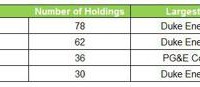
Summary Utilities are a solid income-producing, low volatility plays. Look at utility ETFs as alternatives to one-stock options (Con-Ed, Duke Energy, Dominion) for more geographic and industry diversification. These utilities are largely made in America domestic investment options. Profiling the contenders (unless otherwise stated, market prices, NAV and SEC yield as of 1/23/15) : Vanguard Utilities ETF (NYSEARCA: VPU ) This ETF seeks to track the performance of a benchmark index that measures the investment return of stocks in the utilities sector and includes stocks of companies that distribute electricity, water, gas or that operate as independent power producers. Market price: $106.55 30-day SEC Yield: 3.14% Number of holdings: 78 iShares U.S. Utilities ETF (NYSEARCA: IDU ) This ETF seeks to track the investment results of an index composed of U.S. equities in the utilities sector. Market price: $123.23 30-day SEC Yield: 2.56% Number of holdings: 62 Guggenheim S& P 500 Equal Weight Utilities ETF (NYSEARCA: RYU ) This ETF seeks to replicate as closely as possible, before fees and expenses, the performance of the S&P 500 Equal Weight Index Telecommunication Services & Utilities. Market price: $81.17 30-day SEC Yield: 2.91% Number of holdings: 36 Utilities Select Sector SPDR ETF (NYSEARCA: XLU ) This ETF seeks to provide investment results that, before fees and expenses, correspond generally to the price and yield performance of the S&P Utilities Select Sector Index. Market price $49.14 30-day SEC Yield: 3.04% Number of holdings: 30 1) Diversification Diversification is the process of reducing non-systematic risk by investing in a variety of assets or asset classes that (hopefully) do not move up or down in value at the same time or magnitude. As the 2008 financial crisis taught us , there are certain unforeseeable events (think global recession, world wars) that no amount of diversification can protect us from. With diversification, you are at risk, without it you are doomed. a) Number of holdings An ETF does not need to hold every company of every sector that comprises its benchmark index, but 2 – 3 companies per industry is my subjective minimum to achieve adequate diversification. The utilities sector can be broken up into various industries including: electric utilities, multi-utilities, gas utilities, independent power and renewable electricity providers and water utilities. (click to enlarge) Winner: Guggenheim. While iShares and Vanguard both have more holdings, the concentration of risk with Duke Energy should not be ignored. Every dollar invested in Duke Energy is a dollar that can’t be invested in smaller regional electric and water companies that potentially could provide under the radar value for investors. b) Industry concentration Vanguard Utilities ETF (Courtesy of Vanguard) iShares U.S. Utilities ETF (Courtesy of BlackRock) Guggenheim S&P 500 Equal Weight Utilities (click to enlarge) ( (Courtesy of Guggenheim Investments) Utilities Select Sector SPDR ETF (Courtesy of State Street Global Investors) Winner: Guggenheim. I like that it has three industries that make up 10% or more of total investments, compared to only two for the competition. While diversified telecommunication services sounds a lot like AT&T, Verizon et al, this high barrier-to-entry quasi utility addition adds recurring revenue and relatively higher yield to the mix. 2) Expense ratio The SEC defines expense ratio as the total of a funds operating expenses, expressed as percentage of average net assets. The expenses include management fees, Distribution/service or “12b-1” fees, custodial, legal, accounting, etc. Lower expense ratios, either through larger size or smaller nominal expenses mean higher investment returns. (click to enlarge) Winner: Vanguard. John C. Bogle , founder of Vanguard: The grim irony of investing, then, is that we investors as a group not only don’t get what we pay for, we get precisely what we don’t pay for. So if we pay for nothing, we get everything. Honorable mention: the other three. According to Morningstar data , the average expense ratio for similar funds is 1.28%. 3) Total return (click to enlarge) Winner: Guggenheim. The Guggenheim S&P 500 Equal Weight Utilities ETF has outperformed Vanguard, iShares, and SPDR on both three and five year horizons. Past performance is no indicator of future results, naturally, but I believe this result is indicative of a superior indexing methodology. 4) Valuation multiples Winner: Vanguard. The Vanguard ETF is trading at a slightly lower multiple to TTM earnings, and a reasonable price/book ratio related to its competitors. 5) Liquidity The ability to get out of a great investment is just as important as the ability to get in. While ETFs are generally regarded as having higher liquidity than mutual funds (primarily because they can be traded throughout the day, rather than just at the end), there are reasons to avoid ETFs with excessively low volume. Chief among these are higher bid-ask spreads, which may result in the inability to profitably execute a short-term trade (not a real issue for long-term investors). However, one of the issues that arises from low liquidity (a deviation between price and NAV) can actually be an opportunity. If an ETF is trading slightly below its NAV, but the market is not active enough for it to quickly resume equilibrium, you can shave a few points off your basis by looking for opportune entry points. (click to enlarge) (click to enlarge) Winner: SPDR. Higher volume means tighter bid-ask spreads, full stop. 6) Yield (click to enlarge) Winner: Vanguard. Honorable mention: Everyone else. All four ETF options offer better income producing prospects than a 30 year treasury (2.38%), the S&P 500 (1.97%), and Dow Jones Utility Average (2.40%). 7) Volatility (click to enlarge) Winner: SPDR. Over three and five-year time-frames, SPDR has been less volatile than Vanguard, iShares and Guggenheim, and significantly less volatile than markets as a whole. 8) Dividend history and growth Source: finance.yahoo.com Winner: Tie: SPDR and iShares. The SPDR and iShares ETF have increased their annual dividend each year since 2009. Growing dividend payments is one way to try and keep up with inflation, and based on this 6 year time-frame, SPRD and iShares best accomplish this. So, which Utility ETF should you own? SPDR! The Utilities Select Sector ETF by SPDR is: the most active (liquid), the least volatile, offers the second highest yield, the second lowest expense ratio, and is one of only two of the funds analyzed that has increased dividends each year since 2009. A word of caution Utilities stocks are generally thought of as defensive plays, and could underperform in a rising or bull market. Also, significant sustained changes in the cost of energy production and delivery or interest rates could negatively impact all of these stocks. That is no excuse, however for not considering allocating at least a portion of your portfolio to these low-volatility ETFs. Do your homework, review the composition and risk profile of each of these ETFs and monitor your holdings.
Risk Of Grexit And GLD

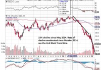
Background of the difficult economic conditions of the eurozone and the threat of Syriza’s victory in Greece. GLD has already priced in the threat of Syriza since November 2014 and has been rising steadily. Those who wants the safe habour of gold has already gone in. Risk of Syriza overtipping its hand for a quick fix to high debt with a primary budget surplus even though there are indications that Syriza will be moderate in power. Time to hold for those with GLD exposure and observe future developments and for those without exposure to initiate it. Difficult Times For The Eurozone Gold has been used been used as a medium of exchange since historic times and especially in times of turmoil. In modern times, with the creation of bank notes and the 1971 closing of the gold window, paper money is the medium of exchange and its power lies in the ‘full faith and credit of’ whichever government that is issuing the note. Now the full faith and credit of the United States Government is still valid in the market especially in a time where the U.S. economy is growing strongly (11 year high of 5% GDP growth in the third quarter of 2014), the U.S. Dollar (USD) is strong and most importantly the state of the union is strong. However the same attributes cannot be said for the eurozone. The eurozone economy is faltering at 0.2% growth for the same third quarter 2014 when the U.S. is growing strongly. The euro, as represented by the CurrencyShare Euro Trust ETF (NYSEARCA: FXE ), has declined by 23% since 05 May 2014 as seen in the chart below and this decline has accelerated since October 2014 which coincided with a dovish European Central Bank (ECB) decision. (click to enlarge) Lastly there is the issue regarding the state of the eurozone. The integrity of the eurozone had been tested in 2012 when Greece almost elected Syriza who came in second into government. This sparks the famous line by ECB President Draghi to ‘do whatever it takes’ to preserve the euro. The Rise and Threat of Syriza on Eurozone Now with the snap General Election on 25 January 2015, Syriza has defeated the previous government New Democracy to form the next government of Greece and its firebrand leader Alexis Tsipras would be youngest Greek Prime Minister at age 40 in 150 years. The whole reason that Syriza poses an existential threat to the whole eurozone project is quite simply because it does not want to pay its huge external debts. Its policy platform is anti-austerity, the repudiation of debt in essence and more social spending. This is what got it in power in the very first place which pleased the Greek population and at the same time send an earthquake to the rest of the eurozone. This whole political instability came about from the failed election of President of Greece. The President of Greece is a largely ceremonial role held currently by the incumbent Karolos Papoulias for 2 terms of 5 years each. His second term is set to end in March 2015. The President of Greece is elected by the Hellenic Parliament in Greece and has to be done latest 1 month before he is set to leave office as decreed by the Greek Constitution. The Prime Minister of Greece Samaras brought it forward to December 2014 but he was unable to secure a 2/3 majority of parliament vote for his candidate on the first 2 rounds of voting on the 17th and 23rd. The third round of voting on the 27th also failed to produce the reduced 3/5 majority of 180 votes which triggered the election for a new parliament on 25 January 2015. The new parliament will have to vote for the new president again by February 2015. Safe Harbor of GLD If you are a rich or middle class citizen (with enough money beyond the hand to mouth existence to be worried) in Europe and you are faced with the possibility that the euro note you hold can either be worthless or in the more optimistic case, be exchanged back at a steep discount to the national currency, what will your natural options be? You will avoid European equities and bonds because they are denominated in euros. You might want to change into a currency like the USD that will hold its value or you might want to buy physical gold which is harder to devalue or you might want to invest into a gold ETF denominated in the USD like GLD to avoid the storage and insurance costs. This is why we can see that the value of gold, as seen in the SDPR Gold Trust ETF (NYSEARCA: GLD ), has rose steadily since 03 November 2014 whenever there is a hint of potential political instability in Greece. (click to enlarge) As we can see, the market is forward looking and has began to price in the Greek instability before the formal vote in the Hellenic Parliament. Gold investors started to buy when the rumor of the a potential change in government given the weakness of the current Greek coalition government. This is why we are unlikely to see a sudden spike up in GLD now because the market has sufficient time to build their long position. Even for those who are less connected, they will have seen in coming last month when the rounds of Presidential election failed in Parliament. History of Debt Concession However now that Syriza has formed the new government,it remains to be seen how far its leader Tsprais will go to fulfill his campaign promises. It is clear that he will want to extract some sort of concession from the Troika. The prior Greek government managed to extend the loan repayment period from the original 7 years to 15 years in July 2011 and interest rates were cut to 3.5% for a mega loan of $109 billion euros loan package. This is the start of the second and ongoing Economic Adjustment Program for Greece after the first program which saw loans of $110 billion euros from May 2010 to June 2011. It is also in this period where we saw a soft default on a debt restructuring deal which concluded on 09 March 2012 on $205.5 billion euro of debt. This caused the ISDA to call a Credit Event which triggered $3.5 billion of credit default swaps and let Fitch to downgrade Greek debt from ‘CCC’ to ‘Restricted Default’. All in all, through this soft default option, Greek debt holders lost a massive $107 billion euros, a record for sovereign debt losses. Is this the calm before or after the Storm? As far as the market is concerned, the eurozone has survived this crisis of soft default with the help of the ECB when other organization were unable to convince the market. This soft default option is therefore unlikely to affect the market drastically. In other words, the extent and pretend scheme coupled with significant haircut works to preserve the eurozone even if it caused dismay to bond holders. Now the market is waiting to see if Syriza will actually dare to defy the Troika and simply walk away from its debt given the consequences. As this Reuters report shows, even as early as 04 November 2014 (coinciding with the rise of gold prices), when Syriza gets closer to power, it has proceeded to soften its stance from the choice of hard default to renegotiation. The German/ Creditor’s position is clear. They are willing to accept a debt restructuring but they will not accept a hard default or any cancellation of debt. This will weaken their position with other debtor countries like Poland, Ireland and Spain. The only risk now is that Syriza will overtip its hand when asking for concessions to the point where it is unacceptable to the Creditors. This is a possibility given the nature of his fiery speech and the expectations of quick relief from the Greek public. (click to enlarge) Source: Google There is a possibility that he will be too engrossed about the quick fix of Greek 175% debt to GDP ratio, which is higher than the rest of Europe. There is also the temptation to turn the Greek’s primary budget surplus of $3.3 billion euros for year 2015 to a current account surplus if they don’t pay off their external debts. The real risk is that Tsprias might then be too willing to leave the eurozone and underestimate the possibility of the hyperinflation tragedy. This might happen when the drachma is reintroduced at a point where the international market has no confidence in it shortly after a massive debt default. Conclusion GLD has appreciated way before the actual victory of Syriza and those who wanted to hold gold already has gold exposure in their portfolio. These are the cautious ones. For the vast majority of the public, it is the fear for systemic unrest on the scale of Lehman Brother collapse that will bring them into gold in doves. This fear will only occur when there are clearer signs of a disorderly Greece Exit (or Grexit). While we believe that Syriza was only posturing to gain power and it might be slightly more aggressive than the outgoing New Democracy government, there is also a serious risk that the inexperienced Syriza will overturn its hand and oversee the expulsion of Greece from the eurozone under its watch. There might be other forces that might tilt the balance inside and outside Syriza towards a cold calculation of benefits and costs that might result in unexpected results. There is still market confidence in the USD and GLD. For those who are upset about the lack of audit for GLD, consider it from the faith and credit angle. Based on the market capitalization of $30.78 billion and last known daily volume of 6.27 million, it is clear that there is market confidence in GLD and you can liquidate it quickly when you need it. However for those in Europe who are worried about capital controls, then it will make sense for them to hold physical gold but they will have to incur cost for storage and insurance. Then there is also the security risk for holding gold against theft or worst. For them, in today’s world without capital controls in Europe, GLD will be a good way to hold their wealth. For investors in general, they would do well to hold onto their GLD holdings especially for those who heeded my earlier advice to buy GLD in my earlier article, The SNB Catalyst For GLD . That article also explored the potential European instability from a different perspective. For those who have nil exposure to GLD, this will be a good time to gain exposure when there will be a brief lull in prices as the market wait and observe the actions of the new Greek government and the official response from the Troika who represent the Creditors.

Does ‘Sharpe Parity’ Work Better Than ‘Risk Parity?’

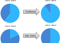
By Wesley R. Gray Strategies employing Risk Parity have been favored by mutual funds and other market participants the past few years. The attraction of risk parity strategies is the great story associated with the approach and the historical performance over the past 30 years has been favorable. However, there is an argument that historical risk parity performance has been driven by leveraged exposure to Treasury Bonds, which have been on an epic tear the past ~30 years. Nonetheless, good stories such as risk parity never die on Wall Street, they merely adapt and overcome. This white paper by UBS highlights skepticism around risk parity and presents a different, but related asset allocation method: Sharpe Parity. Risk Parity Background: As you may recall, risk parity identifies weights that equalize “risk” across asset classes. Let’s first review a simple risk parity example. Here is a visual interpretation of how risk parity works. If we allocate to a 60/40 stock/bond portfolio on a dollar-weighted basis, on a risk-contribution basis, we might be getting 90% of our risk from stocks and 10% of our risk from bonds. Risk parity comes to the so-called rescue. Risk parity suggests that we rejigger the dollar-weighted 60/40 portfolio in such a way that the risk contributions end up being 50% driven by bond exposure and 50% driven by stock exposure. In other words, our “risk contributions” are at parity, hence the title “risk parity.” How does this work in practice using the most basic version of risk parity outlined in the Asness, Frazzini, and Pedersen paper: (click to enlarge) Source: Leverage Aversion and Risk Parity (2012), Financial Analysts Journal, 68(1), 47-59 But UBS Doesn’t like Risk Parity. Why? As per their own research: Risk Parity ignores return and focuses only on risk; Risk Parity uses volatility as the sole measure of risk, while neglecting other credit-related risks, such as default risk and illiquidity; Risk Parity encounters huge drawdowns if bonds and equity sell off together; A low nominal return world makes recovery from risk parity drawdowns difficult. UBS proposes a new asset allocation strategy, which shares some concepts with risk parity, but in their approach risk parity’s “standard deviation” is replaced with an estimate for an asset’s Sharpe Ratio. Here’s an explanation of the concept: “Think about it this way: if asset X has a Sharpe ratio of 2 it means that we have two units of return for 1 unit of risk, while asset Y with a Sharpe ratio of 1 gives us only 1 unit of return for the same amount of risk. In that case we construct a portfolio with the weight for asset X being double the weight of asset Y.” Strategy Background: This approach makes some sense, as it seems to account for return as well as risk. This approach is also in line with modern portfolio concepts such as mean-variance analysis, where investors want to maximize marginal Sharpe Ratios to create the so-called “tangency portfolio” that all MBA 101 students know and love. But how does “Sharpe Parity” stand up to empirical scrutiny? In order to address this question, we compare 4 asset allocation approaches: Equal-weight allocation , an equal-weight allocation with a Simple Moving Average rule , simple Risk Parity , and Sharpe Ratio Parity . Equal-weight (EW_Index): monthly rebalanced equal-weight portfolios. Simple Moving Average (EW_Index_MA): calculate a simple moving average each month (12 month average); if the MA rule is triggered (when the current price > 12 month moving average), buy risk, or else, allocate to the risk-free asset. Risk Parity: follow the simple risk parity algorithm; use a look-back period of 36 months for the “standard” risk parity model. Sharpe Parity: use a look-back period of 36 months for the Sharpe Parity model; if an asset has a negative Sharpe Ratio, this asset’s weight will be 0; note that if all the assets’ Sharpe Ratios are negative, the strategy will allocate 100% to the risk-free asset. Data Description: To test these 4 strategies, we apply them to the “IVY 5” asset classes: SP500 = SP500 Total Return Index EAFE = MSCI EAFE Total Return Index REIT = FTSE NAREIT All Equity REITS Total Return Index GSCI = GSCI Index LTR = Merrill Lynch 7-10 year Government Bond Index (click to enlarge) The “IVY 5” Concept. Click to enlarge. Our simulated historical performance period is from 1/1/1980 to 7/31/2014. Results are gross, and thus do not include the effects of fees. All returns are total returns and include the reinvestment of distributions (e.g., dividends). Data was obtained via Bloomberg. Indexes are unmanaged, do not reflect management or trading fees, and one cannot invest directly in an index. Please see the disclosures at the end of this document for additional information. Sharpe Parity has a slightly higher CAGR. However on a risk-adjusted basis, Equal Weight MA and Risk Parity outperform the Sharpe Parity system, as reflected in their higher sharpe and sortino ratios. The simple moving average technique has the lowest drawdown and the best overall risk-adjusted performance. (click to enlarge) The results are hypothetical results and are NOT an indicator of future results and do NOT represent returns that any investor actually attained. Please see disclosures for additional information. Additional information regarding the construction of these results is available upon request. Does Lookback period matter? Next, we change the look-back period from 36 months to 3 months, which is identical to the lookback period used in the UBS whitepaper. Here’s the result: Sharpe Parity based on a 3 months lookback period has larger CAGR, but also has larger drawdowns, on a monthly, worst case, and cumulative basis. Sharpe and sortino ratios are worse than the 36 month lookback version. (click to enlarge) The results are hypothetical results and are NOT an indicator of future results and do NOT represent returns that any investor actually attained. Please see disclosures for additional information. Additional information regarding the construction of these results is available upon request. Conclusions Based on these results, it seems hard to conclude that Sharpe Parity, particularly with a 3 month look-back period, offers a clear-cut advantage over traditional Risk Parity approaches. In fact, on a risk-adjusted basis, it compares poorly. Based on this analysis, it would appear that simple equal-weight portfolios with trend-following rules have worked better than more complicated risk parity or sharpe parity systems. Original Post