Tag Archives: alternative

SLYV Doesn’t Offer Enough Value For My Portfolio
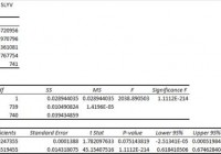
Summary I’m taking a look at SLYV as a candidate for inclusion in my ETF portfolio. The expense ratio is a tad high, but diversification isn’t bad. The correlation with SPY isn’t bad, but the daily returns are more volatile than SLYG. I don’t think I’ll be using SLYV in the foreseeable future. I’m not assessing any tax impacts. Investors should check their own situation for tax exposure. Investors should be seeking to improve their risk adjusted returns. I’m a big fan of using ETFs to achieve the risk adjusted returns relative to the portfolios that a normal investor can generate for themselves after trading costs. I’m working on building a new portfolio and I’m going to be analyzing several of the ETFs that I am considering for my personal portfolio. One of the funds that I’m considering is the SPDR® S&P 600 Small Cap Value ETF (NYSEARCA: SLYV ). I’ll be performing a substantial portion of my analysis along the lines of modern portfolio theory, so my goal is to find ways to minimize costs while achieving diversification to reduce my risk level. What does SLYV do? SLYV attempts to provide results which are comparable (before fees and expenses) to the total return of an unnamed index that tracks small capitalization “value” equity securities in the U.S. By not defining a specific index, it would be difficult for SLYV to fall short of that objective. It may sound like I’m unimpressed with the fund before I even begin the analysis. To an extent, that’s true. I want to see a specific index named so that investors can check how accurately the ETF is tracking that index. I checked the official prospectus to see if there was a mistake. It seems there really is no defined index. SLYV falls under the category of “Small Value”. Does SLYV provide diversification benefits to a portfolio? Each investor may hold a different portfolio, but I use (NYSEARCA: SPY ) as the basis for my analysis. I believe SPY, or another large cap U.S. fund with similar properties, represents the reasonable first step for many investors designing an ETF portfolio. Therefore, I start my diversification analysis by seeing how it works with SPY. I start with an ANOVA table: (click to enlarge) The correlation is about 85.6%, which is great for Modern Portfolio Theory. The lower correlation makes it much easier to mix the ETF into a portfolio and take advantage of the benefits of diversification. My goal is risk adjusted returns, and my method is minimizing risk. Standard deviation of daily returns (dividend adjusted, measured since January 2012) The standard deviation is moderately high, but not terrible. For SLYV it is .9673%. For SPY, it is 0.7300% for the same period. SPY usually beats other ETFs in this regard, and the low correlation with SPY makes the higher standard deviation acceptable. Mixing it with SPY I also run comparisons on the standard deviation of daily returns for the portfolio assuming that the portfolio is combined with the S&P 500. For research, I assume daily rebalancing because it dramatically simplifies the math. With a 50/50 weighting in a portfolio holding only SPY and SLYV, the standard deviation of daily returns across the entire portfolio is 0.8183%. If an investor wanted to use SLYV as a supplement to their portfolio, the standard deviation across the portfolio with 95% in SPY and 5% in SLYV would have been .7354%. Ironically, when I compared the growth version of this fund (NYSEARCA: SLYG ), which is very similar except for investing in “growth” securities, SLYG had lower correlation and a lower standard deviation of returns. I would have expected SLYG to have lower correlation than SLYV, but I would not have expected it to exhibit a smaller standard deviation of returns. In short: SLYV performed worse on both risk metrics than SLYG. Liquidity The average trading volume was a little over 30,000 shares, which is high enough that I’m not concerned. Why I use standard deviation of daily returns I don’t believe historical returns have predictive power for future returns, but I do believe historical values for standard deviations of returns relative to other ETFs have some predictive power on future risks and correlations. Yield & Taxes The distribution yield is 1.36%. The SEC yield is 1.37%. That yield isn’t terrible, but investors won’t be able to retire on yields that are significantly under 2%. In my opinion, this is a difficult space for an ETF to be in. The “value” realm can be associated with less volatility and higher yields which make it more appealing for retirees. This “value” ETF doesn’t have enough yield to be strong in the category but offered more volatility and correlation to SPY than the growth ETF. I’m not a CPA or CFP, so I’m not assessing any tax impacts. Expense Ratio The ETF is posting .25% for an expense ratio. I want diversification, I want stability, and I don’t want to pay for them. The expense ratio on this fund is not too bad, but I’d like to see it lower for an ETF that invests in U.S. equity securities. Market to NAV The ETF is at a .17% premium to NAV currently. Premiums or discounts to NAV can change very quickly so investors should check prior to putting in an order. I wouldn’t want to pay a premium greater than .1% when investing in an ETF, unless I could find a solid accounting reason for the premium to exist. Largest Holdings Just like SLYG, the diversification is fairly solid. No investment is over 1% of the portfolio, but that also isn’t diversified enough to explain the .25% expense ratio. (click to enlarge) Conclusion I’m currently screening a large volume of ETFs for my own portfolio. The portfolio I’m building is through Schwab, so I’m able to trade SLYV with no commissions. I have a strong preference for researching ETFs that are free to trade in my account, so most of my research will be on ETFs that fall under the “ETF OneSource” program. I just don’t see enough benefits to SLYV to try to use it in the portfolio. Due to the low correlation, an investor may find a 1% exposure to be very reasonable. For me, 1% simply isn’t large enough when investing in ETFs. Additional disclosure: Information in this article represents the opinion of the analyst. All statements are represented as opinions, rather than facts, and should not be construed as advice to buy or sell a security. Ratings of “outperform” and “underperform” reflect the analyst’s estimation of a divergence between the market value for a security and the price that would be appropriate given the potential for risks and returns relative to other securities. The analyst does not know your particular objectives for returns or constraints upon investing. All investors are encouraged to do their own research before making any investment decision. Information is regularly obtained from Yahoo Finance, Google Finance, and SEC Database. If Yahoo, Google, or the SEC database contained faulty or old information it could be incorporated into my analysis. The analyst holds a diversified portfolio including mutual funds or index funds which may include a small long exposure to the stock.
Avoid The Value Trap To Achieve Higher Returns

Summary Be wary of value traps in banks, oil and consumer stocks. My sweet attraction to Tootsie Roll goes sour. I paid a premium for my top stocks. Value investors spend their lives in the trenches buying stocks at deep discounts to their peers. They believe their bottom feeding will produce top returns. But sometimes these discounted stocks are a “Value Trap” that never go anywhere. Investopedia says, “The trap springs when investors buy into the company at low prices and the stock never improves. Trading that occurs at low multiples of earnings, cash flow or book value for long periods of time might indicate that the company or the entire sector is in trouble, and that stock prices may not move higher.” There are value traps in all sectors, but I believe traps are common in Oil, Banking and Consumer stocks. I will explore value traps in all three sectors. Candy stocks In the 1990s and 2000s, I had success investing in the William Wrigley Co., achieving 15% annual returns until the stock was sold to Mars at 32 times expected earnings in 2008. I was sad to see that stock leave my portfolio. I looked for other candy companies to purchase. I invested some money in Tootsie Roll (NYSE: TR ). Tootsie Roll has a great story and popular products that are part of American confectionery history, its most well known ad campaign in the 1970s was “How many licks does it take to get to the center of a Tootsie Pop?” The company has solid fundamentals, minimal debt, good cash flow and popular brands. TR trades at a P/E of 29, similar to Hershey (NYSE: HSY ). In the mid 2000s, I bought a few shares of TR at $24 per share, but the stock never went anywhere. I figured some day the Gordon family that owns the majority of stock in Tootsie Roll would eventually sell out and relinquish control. Ellen and Melvin Gordon have run Tootsie Roll for decades and have no plans to step down. After holding my Tootsie Roll stock for a year, I sold the shares for about the same price that I had paid for them. The stock moved to $29.80 per share recently. There is more value in Tootsie Roll, but how long can investors wait for that to be realized? I started buying Hershey stock at around $65 per share. Hershey was up 193% over the past five years compared with 25% for Tootsie Roll. I’m glad I put my money with Hershey. Energy Investors who chased the energy sector seeking deep-discount stocks with fat dividend yields have taken some hits lately. The energy play has produced big-time losses due to the -50% drop in oil prices. Stocks like Sandridge Energy (NYSE: SD ) are hurting. Low oil prices will cut demand for Sandridge’s oil and gas exploration business. SD was down -67% over the past three months. I see many investors looking for an opportunity in Seadrill (NYSE: SDRL ). Seadrill is trading at forward 3.68 P/E and trailing 1.22 P/E. The stock is trading at half of its stated book value. It looks cheap. But a closer look and you see earnings growth is not there. In fact, YOY quarterly earnings growth is a negative -47%. I question SDRL’s $20.93 book value. With oil prices cut in half, the company’s assets are probably worth substantially less at this time. SDRL cut its dividend to save cash. SDRL will lose business in 2015. Who wants to pay for its expensive ocean drilling systems if cheap oil is plentiful on land? Banking I know bankers who really got hammered with the stock market crash in 2008-09. Bank of America (NYSE: BAC ) used to trade over $40 per share in the mid 2000s, but fell to $3.00 per share in 2009. The stock recently hit $16.90 per share, but has never fully recovered its pre-recession share price. Meanwhile if you had owned the S&P500 or (NYSEARCA: SPY ) before, during and after the Great Recession, you would have recovered your principle by 2012 and made phenomenal returns of 32% in 2013 and 13.5% in 2014. BAC is trading at 81% of book value. Citi is trading at around 80% of tangible book value. This may be a classic value trap. Banco Santander S.A. (NYSE: SAN ) is trading around 86% of book value compared with Wells Fargo (NYSE: WFC ) trading at 1.67 times book value. SAN has decided to raise more capital through issuing stock. This will dilute shareholder value. Banks are over-regulated, pay high expenses on legal issues and deal with a low-interest rate environment that makes it difficult to earn money. Regulators want banks to maintain high capital levels. With interest rates so low, banks can’t pay much on savings accounts. Every time you turn around, a lawmaker wants to propose new, tougher standards for banks. Banks already spend a lot of money on internal controls, legal and compliance. Don’t buy bank stocks with the idea interest rates are going up because we may see low interest rates for many more years. The 10-year Treasury actually fell from 3.00% to 2.00% in 2014. U.S. bond yields remain low due to worldwide pressures keeping rates down. The Federal Reserve is in no hurry to raise rates, although it hinted we might see an uptick in rates by summer 2015. If I had waited for deep-discount prices on my favorite stocks, I might not have bought them except in 2009 when all financial assets deflated. I paid a premium for my favorite stocks and bought them on the dips. Now these stocks represent the most consistent and profitable returns in my portfolio. These quality stocks are Berkshire Hathaway (BRK.B, BRK.A), Union Pacific (NYSE: UNP ), Hershey, Church & Dwight (NYSE: CHD ), Boston Beer (NYSE: SAM ) and Dominion Resources (NYSE: D ). I bought these stocks using a multiple-buy-on-the-dips approach that reduced risk and increased my returns. A stock’s value is really dependent on a stock’s future earnings potential. Positive, upside surprises on earnings usually drive stocks higher. If a company produces higher levels of earnings year after year without diluting shares, the stock eventually will move up in price. But if the prospects for earnings growth is taken away, the stock may never appreciate. Conclusion Buy companies that generate large amounts of cash daily, have minimal or no debt and that don’t get in trouble with the government. Watch out for the value trap. I’m staying away from oil and banking stocks to devote more capital to my winners. Don’t chase losers into the hole of no return. Money not lost is money ahead.

Using Adaptive Asset Allocation To Limit Market Risk And Increase Return

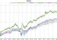
Summary Adaptive asset allocation enables an investor to capture higher returns and reduce risk compared to “buy and hold” and “fixed asset allocation”. Adaptive asset allocation can adjust the portfolio to compensate for varying market conditions. A backtest from Nov 2005 to Jan 2015 shows one allocation strategy resulting in more than double the returns and much less risk compared to a buy and hold strategy. Adaptive asset allocation is often cited as an attractive alternative to fixed or standard asset allocation so popularly used. Standard asset allocation or fixed asset allocation is the idea of allocating 10% of your portfolio to this and 25% to that and another 7% to this asset class and keeping that percentage fixed regardless of market circumstances. Adaptive asset allocation is quite different in how it decides how much is allocated to each asset in a portfolio, instead of using fixed numbers set by an individual or corporation at one time during one market cycle and sticking with it through thick and thin, adaptive asset allocation adjusts or adapts the portfolio weightings on a regular basis based on maximizing or minimizing a certain performance metric such as volatility or variance or even the Sharpe ratio. Market cycles as well as bear markets can be ruinous at worst and challenging at best for most fixed asset allocation models. If you recall 2008, the S&P 500 lost around 55% of it’s value, but Gold didn’t miss a beat until it has lost 1/3 of it’s value from 2011-2013. Bonds surged while the stock market crashed in 2008, but many bonds faltered for much of 2013 while the stock market soared. Certainly you can see why diversifying a portfolio is of great value, but it begs the question “Why did we have to hold on to the stock funds we were invested in?”. The first reason we could cite is a very valid one, and it is because we needed to hold onto it so we could benefit from it in the good years like 2013. The next question you may ask is “Why couldn’t we reduce the amount of money we have in the stock market when it is falling or the bond market when it was falling and why have I been holding so much Gold the last few years?”. This is where a fixed allocation system simply says we set a fixed amount and we stick to it regardless of circumstances, but lets take a look at how adaptive asset allocation answers this question. Enter Adaptive Asset Allocation Adaptive Asset Allocation sets the weight of each asset in your portfolio not by a fixed percentage but as a result of optimizing different performance metrics. For example, we could optimize a portfolio’s weightings to minimize volatility or minimize variance or maximize the risk adjusted return (Sharpe Ratio). Each of these optimization criterion can be used to decide how much of each asset in your portfolio instead of using a fixed percentage. As you can see, adaptive asset allocation answers the questions posed above, namely how can we reduce the allocation in a certain asset when it is doing poorly. We are now going to reduce our assets in an asset that is volatile or has a high variance or a low risk adjust return (Sharpe Ratio), and increase our assets in funds that have low volatility or low variance or a high risk adjusted return. Our Test Now that we have established the rationale for why we might want to use adaptive asset allocation let’s test a sample portfolio to see if Adaptive Asset Allocation can improve returns and reduce drawdown. For this portfolio I am going to use Exchange Trade Funds (ETFs) to select US Stocks, International Stocks, Gold, and US Treasury bonds as our portfolio assets. The tickers used are SPY for US Stocks, EFA for International Stocks, GLD for Gold, and TLT for US Treasury bonds. Parameters We are going to try 3 different performance metrics for deciding our weighting, the first is minimizing volatility, the second is minimizing variance, and the third is maximizing the risk adjusted return (Sharpe Ratio). For all calculations we are just going to use the 3 month trailing volatility, variance, and Sharpe ratio as our measurement. We are going to adjust the portfolio on a monthly basis, this may be too often or not often enough, but for an introduction to these type of ideas it is what we will use. Results – Volatility (click to enlarge) Pink Line is Volatility Returns (click to enlarge) Weightings for each symbol over time (EFA=yellow, GLD=blue, SPY=green, TLT=pink) The performance for the minimum volatility weighted portfolio is: 9.42% CAGR 0.98 Sharpe Ratio 9.72% Volatility 22% maximum draw down This compares to the equally weighted version of this portfolio (25% SPY, 25% GLD, 25% EFA, 25% TLT): 8.5% CAGR 0.76 Sharpe Ratio 11.61% Volatility 28.81% maximum draw down And to the S&P 500 alone: 7.64% CAGR 0.47 Sharpe Ratio 19.96% Volatility 55.22% maximum draw down The minimum volatility adaptive asset allocation portfolio successful outperformed the S&P 500, and equally weighted portfolio in all the performance metrics shown above! As you will see in the transition map image above, the volatility adaptive asset allocation did a lot of what we mentioned to reduce risk; during the 2008 stock market crash the % in SPY and EFA dropped considerably, while the bond fund took over a large percentage of the portfolio, and recently the allocation in gold has been dropping to reduce the exposure to the falling gold market. Results – Variance (click to enlarge) Blue Line is Variance Returns (click to enlarge) Weightings for each symbol over time (EFA=yellow, GLD=blue, SPY=green, TLT=pink) The performance for the minimum variance weighted portfolio is: 10.1% CAGR 1.12 Sharpe Ratio 8.95% Volatility 14.84% maximum draw down The minimum variance adaptive asset allocation portfolio again successful outperformed the S&P 500, and equally weighted portfolio in all the performance metrics shown above! The minimum variance adaptive asset allocation did even more than the minimum volatility portfolio to reduce risk and increase returns. During the 2008 stock market crash the % in SPY and EFA dropped to near 0%, while the bond fund took over the majority of the portfolio, the allocation in bonds dropped while stocks recovered, and recently the allocation in gold has been dropping to near 0% to reduce the exposure to the falling gold market. Results – Risk Adjusted Return (Sharpe Ratio) (click to enlarge) Green Line is Sharpe Ratio Returns (click to enlarge) Weightings for each symbol over time (EFA=yellow, GLD=blue, SPY=green, TLT=pink) The performance for the maximum Risk Adjusted Return (Sharpe Ratio) weighted portfolio is: 15.43% CAGR 1.07 Sharpe Ratio 14.4% Volatility 27.27% maximum draw down The maximum Sharpe ratio adaptive asset allocation portfolio again successful outperformed the S&P 500, and equally weighted portfolio in all the performance metrics shown above – especially returns! The maximum Sharpe Ratio adaptive asset allocation did a lot to increase returns and even managed to outperform in the areas of drawdown and volatility over the S&P 500 and equal weight portfolios. Optimizing the Sharpe ratio is definitely aggressive, you will notice how it often completely eliminates assets from the portfolio and even is only in a single asset during certain times. During the 2008 stock market crash the % in SPY and EFA dropped to 0%, while the bond fund took the entire 100% of the portfolio, the allocation in bonds dropped while stocks recovered and there were many times when stocks where 100% of the portfolio, and recently gold has been almost completely absent from the portfolio even though it played a strong role in the portfolio when it was surging upwards earlier in the backtest. One More Thing… One thing that may be problematic is the fact that some of these allocations involve entirely or nearly getting rid of an investment, especially the Sharpe Ratio portfolio. One thing we can do to combat this is what I call “dampen” the weighting algorithms. This involves “dampening” the effects of each weighting algorithm by only allowing the weighting algorithm to go so far. For example you could decide you want to hold no less than 5% of a certain asset, you could then call 0-4% 5% and adjust the other weightings accordingly to effectively “dampen” the effect of the weighting algorithm to make the portfolio more like a fixed allocation strategy. So lets take a quick look at “dampening” the Sharpe Ratio adaptive asset allocation portfolio to see what a little more conservative switching can do: Results – Risk Adjusted Return (Sharpe Ratio) with ~7% Minimum per Asset (click to enlarge) Green Line is Sharpe Ratio with Dampening Applied (click to enlarge) Weightings for each symbol over time (EFA=yellow, GLD=blue, SPY=green, TLT=pink) The performance for the maximum Risk Adjusted Return (Sharpe Ratio) weighted portfolio with dampening is: 13.68% CAGR 1.13 Sharpe Ratio 12.04% Volatility 24.68% maximum draw down So we reduced the full effect of the Sharpe Ratio weighting and we got a portfolio that did not entirely eliminate any symbol, but also wasn’t afraid to aggressively reduce its allocation in assets when they had a bad risk adjusted return value. The results show a smaller CAGR return %, but improvements in the area of Sharpe Ratio, volatility, and maximum drawdown. Conclusion Adaptive asset allocation can be used to re-weight our portfolio to reduce drawdown and increase returns in the ever changing markets as opposed to a more traditional fixed asset allocation. We tested 3 techniques that can be used to weighted a portfolio and noticed how each responded to the changes in the stock markets, bond markets, and gold market. Each strategy was able to outperform a standard buy and hold approach and the stock market, while also delivering better volatility and draw down numbers in the backtests presented above. With ever increasing uncertainty in the direction of the markets and how best to diversify a portfolio adaptive asset allocation may be one answer of how to eliminate guesswork and provide a foundation for adjusting allocations to compensate for the winds and waves of the markets.