Scalper1 News
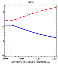
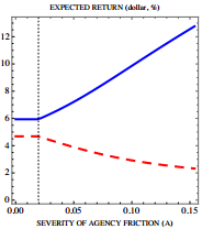 By Jack Vogel, Ph.D. Asset Manager Contracts and Equilibrium Prices Abstract: We study the joint determination of fund managers’ contracts and equilibrium asset prices. Because of agency frictions, investors make managers’ fees more sensitive to performance and benchmark performance against a market index. This makes managers unwilling to deviate from the index and exacerbates price distortions. Because trading against overvaluation exposes managers to greater risk of deviating from the index than trading against undervaluation, agency frictions bias the aggregate market upwards. They can also generate a negative relationship between risk and return because they raise the volatility of overvalued assets. Socially optimal contracts provide steeper performance incentives and cause larger pricing distortions than privately optimal contracts. Core Idea: This is a theoretical paper, so proceed with caution! However, the paper does a good job discussing the Principal/Agent Problem . Briefly stated, the “principal/agent problem” relates to how the interests of agents, who act on behalf of principals, can conflict with those of the principals. In investing, when an asset manager’s performance (or fees) is measured or benchmarked relative to an index, the potential friction (of losing fees and possibly their job) causes the manager to track closer to the index. Here is a quote from the paper: Benchmarking, however, only incentivizes the manager to take risk that correlates closely with the index, and discourages deviations from that benchmark. Thus, the manager becomes less willing to overweight assets in low demand by buy-and-hold investors, and to underweight assets in high demand. The former assets become more undervalued in equilibrium, and the latter assets become more overvalued. Within this theoretical framework, how are asset prices affected? In the graphs below, the blue solid line represents assets in large supply, and the red dashed line assets in small supply. Notice in the graph, that the more expensive asset has lower supply, while the less expensive asset has higher supply! Not surprisingly, the expected return is inverted, where the asset with less supply and is more expensive has lower expected returns, while the asset with high supply and lower price has higher expected returns. Additionally, these assets with higher (lower) supply have lower (higher) volatility. See the paper for details on why this may be so. Note, however, that if an expensive (overvalued) asset with higher volatility has a positive shock to expected cash flows, it would account for a larger portion of market movement. For this reason, managers are reluctant not to hold it, and instead will buy it, since they fear that failing to buy it may cause them to deviate from the benchmark. The main conclusion is that in this theoretical world, asset managers tend to hug the index, as their fees are tied to the index, and thus they are loath to do things that might cause them to depart from it. In the real world, this makes sense as well. Imagine the following two investment strategies that an institutional money manger must pick from: With 98% certainty, you are going to beat the index by 5% over the next 10 years. The other 2% of the time, you will lose to the index by 1%. However, you know that 3 of the years you may lose by as much as 8%! So while the long run expected returns are quite high, the return path to get there is very noisy and volatile. With 50% certainty, you are going to beat the index by 1% over the next 10 years. The other 50% of the time, you will lose to the index by 0.50%. In any given year, you will be +/- 0.25% relative to the index. Here, the long run expected returns are comparatively lower, but the return path is stable. Now, from a mathematical and economist perspective, there is an easy solution — calculate the expected value. Expected Value = beat index by (0.98%)(5%) + (2%)(-1%) = beat index by 4.88% Expected Value = beat index by (0.50%)(1%) + (50%)(-0.5%) = beat index by 0.50 % Any economist would pick option 1! It’s a slam dunk. However, the asset manager knows that picking option 1 is risky to him as an agent, as he might lose his job if the principal (owner of money) loses faith in his strategy. Ever wonder why smart beta products run rampant in the marketplace? It’s because smart beta has low tracking error versus the index. Although expected returns are modest, the manager will remain withing hailing distance of the benchmark, and a principal can’t complain too much about that, right? Unfortunately, this may not necessarily be in the principal’s best interests. Original Post Scalper1 News
Scalper1 News