Tag Archives: portfolio

Structured Notes: Read The Fine Print

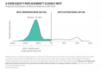
By Seth J. Masters, Richard Weaver, John McLaughlin Structured notes have gained in popularity, but investors would be wise to read the fine print carefully. Our research indicates that these complex instruments rarely live up to their intriguing claims. Nearly $13 billion of structured notes were sold by banks in the first quarter of 2015-more than in any quarter since early 2011. It’s easy to see why. Who wouldn’t like to participate in the equity market’s upside, while protecting their portfolio from potential losses? Unfortunately, our research shows that structured notes seldom deliver the promising outcomes touted in their bold headlines. Structured notes come in many flavors, and we analyzed the claims of several of the more popular varieties. Our analysis found that an oversimplified pitch typically obscures key constraints that adversely impact the investor’s likely final payout. Give with the Left, Take with the Right Consider a recent five-year structured note tied to the broad market that promises the price return of the S&P 500 Index but no loss on the first 28% cumulative drop. Buried in the disclosure are important caveats, including the lack of dividends or yield, plus a five-year waiting period for any distributions. Those who skip the fine print might be tempted to consider this note as a potential replacement for direct stock exposure. In our view, that would be a mistake. Our analysis suggests that this structured note has an 80% chance of underperforming the S&P 500 over the next five years-and by no small amount. Using our Capital Markets Engine, we estimate the median return that investors would forego at just over 12%, as the Display below shows. A closer look under the hood reveals why. To achieve the optimal balance between upside and downside, banks package a zero-coupon bond with options on the S&P 500. In addition to markups on the embedded bond and options, there’s a healthy sales commission, all of which reduce investors’ return potential. Tying the note to the S&P 500’s price return-as opposed to the total return you’d receive through an S&P 500 index fund or ETF-is another drawback. The index fund includes dividends, which have historically been a meaningful portion of the broad market’s overall gains. Missing out on dividends for five years puts the note at a distinct disadvantage. It explains the lion’s share of the performance gap. Settling for Less Given the structured note’s mix of growth and protection, some might consider a balanced portfolio that includes globally diversified equities, municipal bonds and other diversifiers a more relevant comparison. Here again, the structured note falls short. Projecting thousands of plausible outcomes across all types of market environments, we found that the median outcome for the structured note is more than 6% below what we’d expect from a fully diversified balanced portfolio, as the next Display shows. Given the sales pitch, you might expect the structured note to do better if the S&P 500 price declines over five years. Not so! In down markets, the structured note would protect you from losses up to 28%, but your expected return would be zero. By comparison, we forecast that a balanced portfolio that includes bonds and other diversifiers would have an expected return of 4.5%, with better downside protection from a deeper market drop. That’s because the income from bonds-along with their tendency to move in the opposite direction from equities-can help offset the losses from stocks, while alternatives act as a further diversifier. In short, if investors are willing to accept no return, they are setting the bar too low. For most investors, an income-generating balanced portfolio that is both liquid and likelier to outperform represents a much better solution. When it comes to structured notes, investors need to make sure they’re getting the full picture from their provider. The views expressed herein do not constitute research, investment advice or trade recommendations and do not necessarily represent the views of all AB portfolio-management teams. The Bernstein Wealth Forecasting System uses a Monte Carlo model that simulates 10,000 plausible paths of return for each asset class and inflation and produces a probability distribution of outcomes. The model does not draw randomly from a set of historical returns to produce estimates for the future. Instead, the forecasts (1) are based on the building blocks of asset returns, such as inflation, yields, yield spreads, stock earnings and price multiples; (2) incorporate the linkages that exist among the returns of various asset classes; (3) take into account current market conditions at the beginning of the analysis; and (4) factor in a reasonable degree of randomness and unpredictability.

The 4% Spending Rule: Golden Rule Or Guideline?

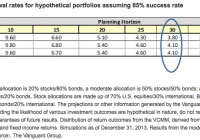
Summary Today’s environment of high equity valuations and low interest rates shouldn’t be ignored. Are investment costs a factor, and if so, how much? Embrace a dynamic spending strategy that considers market performance and allows for flexibility each year. By Maria Bruno, CFP Hardly, a week goes by without seeing some type of headline news discussing the viability of the venerable 4% spending rule. Indeed a simple internet search will yield more than 5 million results! It’s no wonder that retirees may be more confused now than ever. It’s hard to believe that 20 years have passed since William Bengen published his research about sustainable retirement withdrawal rates.[1] During this time, many researchers (including those at Vanguard) have discussed, debated, and continued to crunch the numbers. Much has occurred in the capital markets, including three bull markets, two bear markets, and historically low fixed income yields. Given the milestone anniversary, it’s a good time to reflect, and there’s no better way to start than by defining what the guideline means. Simply put, the 4% spending guideline stated that retirees with a diversified portfolio split between stocks and bonds could safely withdraw 4% of their initial balance at retirement, adjusting the dollar amount for inflation each year thereafter. This level of spending was intended to provide a stable, inflation-adjusted income stream that had a strong likelihood of being sustained for 30 years, based on historical returns for stocks and bonds. Why does the 4% spending rule get a bad rap? First, much of the earlier research was based on modeling of historical asset class returns. While this approach has its merits, the major limitation is that it doesn’t consider current market and economic conditions. In today’s environment of elevated equity valuations and sustained low interest rates, these factors can’t be ignored. To that end, Vanguard’s research incorporates the current market and economic environment in its long-term projections. (See Figure 1.) Second, most well-thought-out research frames the 4% target as a rule of thumb with trade-offs. As with anything in financial planning, guidelines are a starting point and shouldn’t be taken as much more than that. Retirees need to consider their own personal situations when in managing longevity risk-such as their goals, planning horizon, portfolio composition, and comfort level with “stress testing” different market and spending scenarios. Third, the rule of thumb assumes a dollar inflation-adjusted spending program. This means that, at retirement, the retiree spends 4% of his or her portfolio and adjusts that amount annually for inflation. In reality, very few retirees actually stick with such a strict policy. Further, and more important, following an inflation-adjusted spending strategy exposes the retiree to “sequence of returns” risk. With such a model, the spending amount is adjusted annually for inflation but completely ignores portfolio performance. In periods of sustained poor market performance, particularly at the onset of retirement, the retiree is actually spending a greater percentage and, if left unchecked, exposes the portfolio to premature depletion. Indeed, this is one of the major risks of the 4% spending rule. Sure, costs matter, but how much? Many of the published studies show simulated outcomes using benchmark returns as a proxy, with no consideration of real-life costs such as taxes and investment fees. In our studies, we further analyzed hypothetical cost scenarios to stress test portfolio durability using the 4% spending guideline. In the chart above, we highlighted sustainable withdrawal rate durability at an 85% success rate, meaning that in 85% of the simulations the portfolio lasted for at least 30 years. We simulated reductions for cost-0 cost represents the benchmark, 0.25% represents a lower-cost portfolio, and 1.25% represents a higher-cost portfolio (see Figure 2). The results are rather eye-opening. For a moderate investor, the success rates drop from 84% to 74% when higher costs were used. What this means is that the risk of running out of money moved from a 16% to 26%, and the sole factor was investment costs, which is one of the main things that investors can control! No doubt that spending in retirement will continue to be at the forefront of retirees’ minds for the next 20 years. Here’s how I suggest retirees approach the 4% spending rule. First , they should maintain the perspective that this type of analysis should only be used as a modeling tool to help gauge portfolio durability simulations, assuming you maintain a balanced and diversified portfolio. Second , portfolio management costs are a “drag” on their spending, so it’s important to minimize investment costs and follow a tax-efficient portfolio spending approach. Third , they should embrace a dynamic spending strategy that considers market performance and allows for flexibility on an annual basis. Certainly, these three principles are general in nature, but they can provide investors with a nice tailwind as they head into retirement. I’d like to thank my colleagues Michael DiJoseph and Yan Zilbering for their contributions to this research. For more information on dynamic spending, see Vanguard’s research . Footnotes William P. Bengen, 1994. Determining withdrawal rates using historical data. Journal of Financial Planning (October):171-180. Notes IMPORTANT: The projections or other information generated by the Vanguard Capital Markets Model regarding the likelihood of various investment outcomes are hypothetical in nature, do not reflect actual investment results, and are not guarantees of future results. VCMM results will vary with each use and over time. The VCMM projections are based on a statistical analysis of historical data. Future returns may behave differently from the historical patterns captured in the VCMM. More important, the VCMM may be underestimating extreme negative scenarios unobserved in the historical period on which the model estimation is based. All investments are subject to risk. There is no guarantee that any particular asset allocation or mix of funds will meet your investment objectives or provide you with a given level of income. Diversification does not ensure a profit or protect against a loss in a declining market. The Vanguard Capital Markets Model® is a proprietary financial simulation tool developed and maintained by Vanguard’s primary investment research and advice teams. The model forecasts distributions of future returns for a wide array of broad asset classes. Those asset classes include U.S. and international equity markets, several maturities of the U.S. Treasury and corporate fixed income markets, international fixed income markets, U.S. money markets, commodities, and certain alternative investment strategies. The theoretical and empirical foundation for the Vanguard Capital Markets Model is that the returns of various asset classes reflect the compensation investors require for bearing different types of systematic risk (beta). At the core of the model are estimates of the dynamic statistical relationship between risk factors and asset returns, obtained from statistical analysis based on available monthly financial and economic data from as early as 1960. Using a system of estimated equations, the model then applies a Monte Carlo simulation method to project the estimated interrelationships among risk factors and asset classes as well as uncertainty and randomness over time. The model generates a large set of simulated outcomes for each asset class over several time horizons. Forecasts are obtained by computing measures of central tendency in these simulations. Results produced by the tool will vary with each use and over time.

The Low Volatility Anomaly: Risk Parity

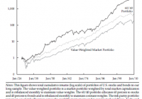
Summary This series offers an expansive look at the Low Volatility Anomaly, or why lower risk securities have historically produced stronger risk-adjusted returns than higher risk securities or the broader market. After examining the historical evidence of the outperformance of lower volatility stocks and bonds relative to their higher risk comps, this article examines a cross-market strategy. The long-run success of risk parity investing is closely linked to our previously discussed Leverage Aversion Hypothesis. In previous articles in this series, I have demonstrated the presence of the Low Volatility Anomaly in both the equity and fixed income markets. In the introductory article to this series , I demonstrated that a low volatility bent (NYSEARCA: SPLV ) to the broader equity market has outperformed both the broader market (NYSEARCA: SPY ) and high beta stocks (NYSEARCA: SPHB ) on both an absolute and risk-adjusted basis over the last quarter century. In the last article in this series , I demonstrated that lower levered BB rated bonds have produced higher absolute returns than higher levered single-B and CCC-rated bonds historically, as the higher yields on the lower rated securities failed to make up for their higher realized default rate. Our empirical evidence thus far has examined the Low Volatility Anomaly within distinct asset classes. This article examines a potential application across asset classes. Risk Parity A 2012 research paper by Clifford Asness, Andrea Frazzini, and Lasse H. Pedersen, ” Leverage Aversion and Risk Parity ” demonstrates that in an investment landscape characterized by, at a minimum, declining incremental returns for higher risk assets, then an approach to asset allocation, risk parity investing, that seeks to diversify in terms of risk and not dollars is preferable. To diversify by risk, more money is invested in low-risk/low volatility assets than in high risk/high beta assets, and leverage is applied to low risk assets to increase both expected returns and risk to its desired level. (If this sounds familiar to the aforementioned ” Betting Against Beta ” analysis, note the overlap in two of the authors.) In their study with data dating to 1926 (see below), the authors demonstrated that a portfolio that targets an equal risk allocation between bonds and stocks meaningfully outperforms 1) U.S. stocks and bonds weighted by total market capitalization, and 2) a portfolio rebalanced monthly to maintain a fixed 60%/40% stock/bond weighting. A preference for risk parity investing necessarily implies expected stock returns continue to produce an insufficiently high equity risk premium as was witnessed by the underperformance of the equity market relative to levered fixed income in the historical sample depicted above. The ballyhooed equity risk premium ( Mehra and Prescott 1985 ), like the risk premium attributable to high beta stocks, is negative in this data over this time horizon featuring multiple business cycles. This phenomenon has given rise to this notion of risk parity investing, a method of diversifying by risk rather than dollars in equities and bonds. This of course runs counter to the traditional notion of holding the market portfolio levered according to the investor’s risk profile instilled by the Capital Asset Pricing Model (CAPM), the model we have been exposing throughout this series. Our first hypothesis for the presence of the Low Volatility Anomaly detailed in this series was the Leverage Aversion Hypothesis . If higher risk-adjusted returns can be made through leveraged fixed income than holding un-levered equities, then risk parity can be viewed as another form of exploitation of the Low Volatility Anomaly. Disclaimer My articles may contain statements and projections that are forward-looking in nature, and therefore, inherently subject to numerous risks, uncertainties and assumptions. While my articles focus on generating long-term risk-adjusted returns, investment decisions necessarily involve the risk of loss of principal. Individual investor circumstances vary significantly, and information gleaned from my articles should be applied to your own unique investment situation, objectives, risk tolerance, and investment horizon. Disclosure: I am/we are long SPLV, SPY. (More…) I wrote this article myself, and it expresses my own opinions. I am not receiving compensation for it (other than from Seeking Alpha). I have no business relationship with any company whose stock is mentioned in this article.