How Do Fidelity’s New Bond Exchange-Traded Funds Stack Up?
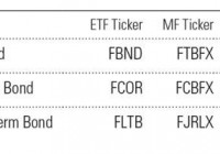
A version of this article was published in the November 2014 issue of Morningstar ETFInvesto r. Download a complimentary copy of ETFInvestor here . On Oct. 9, Fidelity launched three active-bond exchange-traded funds: Fidelity Total Bond (NYSEARCA: FBND ) , Fidelity Corporate Bond (NYSEARCA: FCOR ) , and Fidelity Limited Term Bond (NYSEARCA: FLTB ) . The table below shows the lead managers of each fund as well as their mutual fund analogs. All six funds charge 0.45%. Fidelity follows PIMCO in launching active-bond ETFs, inviting comparison between the two. Are these new funds better than existing PIMCO ETFs? Or passive funds? Fidelity Versus PIMCO Fidelity is more known for its equity funds, but Morningstar analyst Sarah Bush writes that its bond team is “among the industry’s best.” PIMCO is synonymous with fixed income, and analyst Eric Jacobson writes that the firm “[boasts] world-class practitioners and intellects across the board.” So investors have two good options. One big difference between the firms is that PIMCO makes big macroeconomic calls, whereas Fidelity’s bond funds won’t. Most Fidelity bond funds keep their durations close to their benchmarks and focus on making security- and sector-level credit bets. As a consequence, some of Fidelity’s bond funds failed to sidestep the subprime crisis and the financial crisis and suffered sharp losses relative to their benchmarks. PIMCO’s funds, however, sailed through relatively unscathed, having avoided subprime exposure. On the other hand, PIMCO suffered sharp losses in 2011 when it incorrectly bet against Treasuries; Fidelity’s bond funds made no such dramatic calls. Historically, PIMCO’s extensive use of factor timing meant that its fund’s patterns of excess returns relative to their benchmarks were less predictable than Fidelity’s bond funds, which tend to do well when credit does well. Fidelity Total Bond Ford O’Neil is lead manager of both FBND and its mutual fund counterpart, Fidelity Total Bond (MUTF: FTBFX ) . Naturally, the ETF itself can’t be assessed with confidence, but we can make reasonable inferences about its prospective behavior by looking at the mutual fund version of the strategy. O’Neil has spent almost 10 years running the mutual fund, so we have a lot of data to work with. Here’s how Bush describes Fidelity Total Bond’s process: This wide-ranging fund has a variety of tools at its disposal. As at other Fidelity bond funds, duration (a measure of interest-rate sensitivity) is kept close to that of the fund’s bogy, the Barclays U.S. Aggregate Bond Index. Instead, manager O’Neil seeks to beat this benchmark over a three-year period by identifying relatively underpriced sectors of the market and segments of the yield curve, and through individual security selection. This is primarily an investment-grade portfolio–think high-quality corporate bonds, agency mortgages, and Treasuries–livened up with a mix of junk bonds, floating-rate bank loans, and developed- and emerging-markets debt. The fund gets its bank-loan and mortgage exposure from internally run Fidelity “central” funds run by other managers; bank loans are relatively illiquid, so the central-fund approach helps control cash flows, while O’Neil argues that there are significant advantages of scale in the mortgage portfolios. Since O’Neil took over, the fund beat its benchmark by 0.48% annualized as of Sept. 30, 2014. Of course, you can’t own the index. When compared against Vanguard Total Bond Market Index (MUTF: VBMFX ) , O’Neil looks a bit better, extending his edge to 0.61% annualized. However, we care about returns in excess of risk taken. The next chart shows Fidelity Total Bond’s cumulative wealth ratio versus Vanguard Total Bond Market Index. When the line slopes up, Fidelity’s fund is outperforming the Vanguard fund; when it slopes down, it’s underperforming. Total Bond did outperform over O’Neil’s tenure, but at the cost of a nasty drawdown that showed up during the financial crisis. We can get a fuller picture of O’Neil’s record by examining his tenure at Fidelity Intermediate Bond (MUTF: FTHRX ) , which covered July 13, 1998, to Oct. 29, 2013. It is the oldest and longest U.S. bond fund track record of his that we have. The second chart shows cumulative wealth of the fund against its benchmark, the Barclays Intermediate U.S. Government/Credit Index. We see benchmark-matching performance punctuated by a nasty drawdown during the financial crisis. What accounted for these drawdowns? First, O’Neil kept a slug of his fund in an internally managed ultrashort bond portfolio that had substantial exposure to subprime mortgages, which led to the fund’s lagging in late 2007. Second, the fund also had a junk-bond sleeve going into the crisis, but the index excludes them. Despite O’Neil’s mixed record versus his benchmarks, Fidelity Total Bond outpaced most of his category peers, landing in the top 22% for the 10 years ended Sept. 30. The Fidelity Total Bond mutual fund has a Morningstar Analyst Rating of Gold, which indicates Morningstar believes the fund will beat its category peers on a risk-adjusted basis over a full market cycle. There is only one other actively managed ETF of note benchmarked against the Aggregate Index: PIMCO Total Return Active (NYSEARCA: BOND ) , which serves as my default broad bond exposure. The only sensible way to assess investments is through the lens of opportunity cost. Am I giving up space that could be devoted to a better fund if I stick with BOND? I’m about as confident as can be that BOND can beat its benchmark over a full interest-rate or credit cycle, without taking on much more risk. The next chart shows PIMCO Total Return’s cumulative wealth ratio versus the benchmark juxtaposed with Fidelity Total Bond’s cumulative wealth ratio. The different performance patterns reveal the distinct processes driving each fund. PIMCO Total Return is willing to make big macro calls–market-time, in other words–hence its sidestepping much of the carnage of the financial crisis, riding the mortgage-backed securities wave, then getting clobbered in 2011 on its big short Treasury bet. Fidelity Total Bond mostly makes security- and sector-level calls without varying its duration or taking too much risk off the table. The result is the fund that took a beating during the crisis but has steadily earned excess returns as credit exposure has done well. Fidelity Corporate Bond Michael Plage and David Prothro comanage this fund. Although Plage is lead manager of FCOR, Prothro is lead of the mutual fund Fidelity Corporate Bond (MUTF: FCBFX ) . Neither Plage nor Prothro have O’Neil’s long track record. Plage joined Fidelity in 2005 as a fixed-income trader before switching to a portfolio-management role in 2010. Prothro has been with Fidelity as a fixed-income analyst since 1991, but his oldest pure U.S. bond mandate also begins in 2010. Plage and Prothro have done very well with Fidelity Corporate Bond. They’ve beaten their benchmark, the Barclays U.S. Credit Index, by more than 1%. So far it seems as if Plage and Prothro have what it takes. But we haven’t gone through a full credit cycle, so I’m not willing to assign a high degree of confidence that their fund will outperform. There is no other actively managed bond ETF also benchmarked to a similar index or in the corporate-bond category. Fidelity Limited Term Bond FLTB, led by Robert Galusza, begs natural comparisons with the mutual fund Fidelity Limited Term Bond (MUTF: FJRLX ) , also managed by Galusza. The mutual fund’s track record is utterly misleading. A closer look reveals that Fidelity Limited Term Bond until very recently was the Fidelity Advisor Intermediate Bond Fund, which was benchmarked to the Barclays U.S. Intermediate Government/Credit Bond Index. Its lead manager was also O’Neil, who began managing the fund the same day he took over Fidelity Total Bond and ended his tenure on Oct. 29, 2013. Now we have another angle to assess Fidelity Total Bond. Unfortunately, during O’Neil’s tenure, Fidelity Advisor Intermediate Bond underperformed its benchmark with much more volatility. A more relevant mutual fund equivalent for Fidelity Limited Term Bond is Fidelity Short-Term Bond (MUTF: FSBFX ) , which Galusza joined on July 12, 2007. However, Andrew Dudley managed the fund until Feb. 21, 2008. In order to give Galusza the benefit the doubt, I’ll assess his performance the month after Dudley left. The chart shows how he did against the fund’s benchmark, the Barclays U.S. 1-3 Year Government/Credit Bond Index. Like Fidelity Total Bond, Fidelity Short-Term Bond took a big hit during the financial crisis due to its subprime mortgage exposure. Of all three funds, this one is the least appealing from a historical risk/return perspective. It’s also going up against extremely stiff competition in the form of high-yield, low early withdrawal penalty five-year bank CDs that offer 2% yields as of this writing. No ETF offers anywhere near as favorable a risk/reward trade-off. I’ve been consistent in pointing out that low-duration funds are a bad deal, including the two other active ETFs benchmarked to the Barclays U.S. 1-3 Year Government/Credit Bond Index: AdvisorShares Newfleet Multi-Sector Income (NYSEARCA: MINC ) and PIMCO Low Duration Active (NYSEARCA: LDUR ) .