Tag Archives: load

Stock Market Reversal In January: The Potential Effect Of Capital Gain Taxes

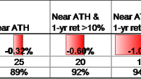
The S&P 500 index was up 11% in 2014 and up 64% over the past 3 calendar years before dividends. When the stock market is at or near all-time highs at the end of December the following January has on average posted a negative return. This reversal effect, likely due to delayed selling because of capital gains taxes, is stronger when the recent 1-year and 3-year returns are high. The past three calendar years have been quite good for the US stock market. Using S&P 500 index data from Yahoo Finance we have only seen better returns for three consecutive calendar years in the late 1990s and the mid-1950s. The S&P 500 data we use begins with full calendar year data in 1951, so we have 63 calendar years of data in our sample through 2013. What can we expect going forward for the stock market or more specifically the S&P 500 index ETFs, (NYSEARCA: SPY ), (NYSEARCA: IVV ), and (NYSEARCA: VOO ), after such a great run? It’s hard to come to any significant conclusions with just five data points, so we want to expand the sample size a bit before analyzing the data. One distinction we can make for this year versus the average year is that we are at all-time highs for the S&P 500. On a monthly closing basis the all-time high was in November with the S&P 500 closing at 2067. December’s close of 2058 is basically right there. There are 25 calendar years in our data set where the December closing level is within 2% of the all-time high. That is enough data to start to draw some conclusions. If we filter this some more by removing years where the last calendar year price change (return before dividends) was less than +10% we have 20 data points. Filtering with a +15% price change gives us 16 data points. We use price change rather than total return because returns from dividends don’t affect decisions about whether to take capital gains or not. The results of various filters are shown in the table below. In the filter criteria, “Near ATH” means December close is within 2% of the monthly closing all-time high, “1-yr ret” means the price change over the prior calendar year, and “3-yr ret” means the price change over the prior three calendar years. (click to enlarge) The confidence level in the last row of the table is a statistical measure that tells us the likelihood that the average January return of each subset of years is actually lower than the typical January return and the difference is not just due to statistical noise. In other words looking at the “Near ATH” column in the table we see there is an 89% chance that Januaries that begin near the all-time high for the S&P 500 can be expected to be worse than the typical January. While this doesn’t pass common statistical tests than require 95% or 99% confidence, it is still worth keeping in mind as investors consider what to do with their portfolios in the New Year. The filter that most closely matches the current environment is the far right column. There have been 11 years since 1951 that end near all-time highs, had greater than +10% price change and finish a three-year period with price change greater than 40%. The subsequent Januaries average price return was negative at -1.11%. The standard error on this sample mean estimate is 1.45%, so while the -1.11% seems significantly different from +0.89% (the average of all years), the difference between the two numbers isn’t that much more than the standard error. The eleven years that match this criteria are shown in the following table. Six out of 11 years are down in January and five are up. The best January in the table follows 1998 with a +4.0% return and the worst follows 1989 with a -7.1% return. Clearly the one year variation is fairly wide, so we can’t expect this January to have exactly a -1.11% decline. How should an investor use this information? Here are a few possibilities. If she wants to add to her equity position, waiting until February might be wise. If rebalancing is in order for a portfolio, and that involves reducing equity exposure, do it sooner rather than later. If it involves adding to equity exposure, wait a month. If there are capital gains in a taxable account and there is any need for the cash this year, sell sooner in January rather than later. If this potential January reversal takes place before an investor can act, it’s probably not a good idea to sell equities out of fear of further declines. For the months of February and March following the eleven Januaries in the table above the combined average returns were +4.1%. We can’t expect this January reversal phenomenon to persist into February and March. We attribute this reversal of returns in January to the impact of capital gains taxes, and delayed selling over the recent past to delay the capital gains tax until April 2016. There could always be some other reason for further selling, or for buying that overwhelms the tax impact to give us a positive return in January. There are a lot of possibilities for what happens to markets in January and in all of 2015. This is just another piece of data to consider that we view as important in the next month. Now that you’ve read this, are you Bullish or Bearish on ? Bullish Bearish Sentiment on ( ) Thanks for sharing your thoughts. Why are you ? Submit & View Results Skip to results » Share this article with a colleague

Now Long Gold And Natural Gas For The 1% Portfolio

This portfolio requires ongoing attention and management. We must justify the extra time invested by producing solid gains. Investing small is imperative in this portfolio. We keep diversified and our investing automatic to control fear and greed. We were put shares of (NYSE:GDXJ) & (NYSE:UNG) over the Christmas. We will monitor these closely and sell covered calls when the opportunity arises. It’s good to be back after the break and I want to wish everyone a very happy new year and let’s work together to ensure 2015 is a very profitable year for all of us. I hope each and every one of you will pick up some ideas and strategies from our 1% portfolio as we march into 2015. We have called this the “1% portfolio” so that the focus is on position size. I understand that it is very difficult for a portfolio to have 100 different underlyings but this portfolio always strives to increase the amount of positions as this has many distinct advantages. As we are starting the year off, let’s go through how this portfolio is set up and also where we are exactly with the 1% portfolio after the Christmas break. First of all this is an income portfolio. Our goal as income investors is to make money every month. We do this through option selling (puts and calls) and dividend pay-outs. This portfolio requires ongoing management because we monitor when an underlying has earnings, when it pays its dividend, when option premium is inflated and obviously the price action of the underlying. If you are looking for a portfolio that it almost completely hands off, then this portfolio is not for you. We are looking for above average gains – at least 25% on our money every year. We need at least this to justify the time we invest in our portfolio management. Investors who don’t want to actively manage their portfolios should just buy some good blue-chips stocks and collect the dividends every quarter as this strategy should overtime give you 7-10% on your money but we want more and the strategies below is how we do it. Firstly we keep our positions very small. Selling covered calls is a good strategy when there is rich option premium in the underlyings but greed creeps in when the underlying rallies hard. When emotions get involved, trading can get reckless. We control this by keeping our positions small and staying diversified. You are never going to “miss” a windfall when you are small and also one position can’t bankrupt you if you remain small in your portfolio. Nevertheless having multiple positions brings its own complexities. When investing small and investing for income, more time must be invested and also we must research the fundamentals of more underlyings. This is where an investor could slip up in this type of portfolio. Instead of doing thorough due diligence, an investor may open a position in an underlying just to collect a dividend which is not what we advocate here. Everything must be lined up properly for this portfolio to be profitable especially the fundamentals of the respective underlying. Secondly in order to collect income, we must sell at a profit. Therefore again when we open option, stock & ETF positions, we put in automatic orders (Good Till Cancelled) to collect income. It is all automatic and we put in these orders at order entry. These orders are working 24/5 for you and their sole aim is to collect income. Moreover these orders take the fear and greed elements out of your trading. We trade on logic not on emotion. When investing in ETFs , we are extremely mindful of where we are in all asset classes. Below is a list of where we believe we are currently in these asset classes. We diversify as much as we can. 1. Agricultural commodities. Corn, Wheat and Sugar are extremely depressed on a historical basis. We will be taking bullish positions in these when the opportunity arises. 2. Precious Metals – Again oversold, especially the mining sector. We will be taking bullish positions in these when the opportunity arises 3. US Equities – Overbought on a historical basis. We only will be going long on our selected blue chips at these levels (Stocks that have flourished historically). If we get a sharp correction, we will add more equities to the mix. 4. Real estate. We believe we are nearing a top in this asset class. We will not be going long here. 5. US Bonds. We believe again that bonds are overbought and are definitely due a correction. We are mindful that this correction may not take place for a substantial period of time. Nevertheless we will not be going long as the risk does not justify the reward at these levels. We made some profits on Coca-Cola (NYSE: K ) over the Christmas period and we also got put stock such as (NYSEARCA: GDXJ ) & (NYSEARCA: UNG ). We will wait until these recover somewhat before we sell some covered calls. We never should have realized losses in this portfolio as we never sell our underlyings at a loss. All we should have should be realized gains and unrealized gains or losses. Updated Portfolio (02-01-2015) Open Positions (Position size kept Ultra Small) Underlying Strategy Result GDXJ – 19/11/2014 Sold 25-DEC26 Naked Put (Now Long Stock) Open UNG – 20/11/2014 Sold 21-DEC26 Naked Put (Now Long Stock) Open USO – 25/11/2014 Sold Jan02-27.5 Naked Put Open USO – 10/12/2014 Sold Jan16-22 Naked Put Open MCD – 17/12/2014 Sold Jan15-95 Covered Call Open KO – 11/12/2014 Sold Jan23-43.50 Covered Call Open CVX -19/12/2014 Bought Stock 19/12/2014 Open CORN – 15/12/2014 Bought Stock – 15/12/2014 Open GDX Bought Stock 09/12/2014 Open MCD Bought Stock 25/11/2014 Open KO Bought Stock 25/11/2014 Open K Bought Stock 25/11/2014 Open TBT Bought Stock 28/11/2014 Open KOL Bought Stock 25/11/2014 Open AXP Bought Stock 05/12/2014 Open BDX Bought Stock 05/12/2014 Open IBM Bought Stock 05/12/2014 Open Closed Positions (Per One Lot Of Options Sold) Underlying Strategy Result GDXJ – 17/11/2014 Sold 22-DEC26 Naked Put $38 Profit MCD – 20/11/2014 Sold 94-DEC26 Naked Put $48 Profit KO – 20/11/2014 Sold 43-DEC26 Naked Put $21 Profit MCD – 16/12/2014 Sold Jan15-95 Covered Call $25 Profit AXP – 16/12/2014 Sold Jan9-95 Covered Call $44 Profit K – 30/12/2014 Sold Jan16-67.5 Covered Call $67 Profit MCD – 15/12/2014 Dividend $0.85 KO – 15/12/2014 Dividend $0.305 K – 15/12/2014 Dividend $0.49

2014 Portfolio Review – What Strategies Worked And Didn’t Work

2014 is officially in the books. And while I don’t like to put too much emphasis on one year of performance, it’s always helpful to look at what has worked and what hasn’t worked. After all, if you want to know where we’re going, it’s often helpful to know where we’ve been. So let’s take a look at some of the more popular portfolio constructions and see how they did in 2014: Global Financial Asset Portfolio (see construction here ) Total Return: 9.24% Standard Deviation: 5.64 Sharpe Ratio: 2.13 S&P 500 Total Return: 13.46% Standard Deviation: 11.53 Sharpe Ratio: 1.74 MSCI EAFE Total Return: -4.5% Standard Deviation: 13.22 Sharpe Ratio: 0.53 MSCI Emerging Markets Index Total Return: 0% Standard Deviation: 15.3 Sharpe Ratio: 0.75 US Long-Term Government Bonds (NYSEARCA: TLT ) Total Return: 27.31% Standard Deviation: 7.49 Sharpe Ratio: 2.93 Zero Coupon Bonds (NYSEARCA: EDV ) Total Return: 42.31% Standard Deviation: 11.19 Sharpe Ratio: 2.99 Goldman Sachs Commodity Index Total Return: -31.2% Standard Deviation: 16.32 Sharpe Ratio: -1.14 Gold Total Return: -3.75% Standard Deviation: 14.16 Sharpe Ratio: -0.32 Silver Total Return: -21.68% Standard Deviation: 25.32 Sharpe Ratio: -0.96 The big winners were US stocks and bonds while the big losers were foreign stocks and commodities. As I’ve long expected, the “high inflation is coming” trade just continued to get clobbered in 2014. The Global Financial Asset Portfolio was a strong performer in general and beat most portfolios on a risk adjusted and nominal basis. Let’s see how the so-called “passive indexing” strategies performed: US 60/40 Stock/Bond Portfolio Total Return: 10.48% Standard Deviation: 6.79 Sharpe Ratio: 2.08 Global 60/40 Stock/Bond Portfolio Total Return: 3.85% Standard Deviation: 8.15 Sharpe Ratio: 1.24 Betterment 60/40 Portfolio (see here for construction) Total Return: 6.48% Standard Deviation: 7.4 Sharpe Ratio: 1.54 WealthFront Aggressive Portfolio (see here for construction) Total Return: 4.83% Standard Deviation: 11.73 Sharpe Ratio: 1.15 Boglehead 3 Fund Portfolio Total Return: 6.91% Standard Deviation: 7.21 Sharpe Ratio: 1.58 Those are some pretty surprising numbers. Given the returns of the GFAP these are all pretty poor figures with the exception of the US focused 60/40. Not surprisingly, the Robo Advisor portfolio actually result in portfolio degradation as I suspected they would when I first analyzed them earlier this year. I still fail to understand why anyone would pay 25 bps or more for these “passively” managed Robo portfolios especially given the obviously misleading claims that their portfolios generate an “estimated additional return” of 4.6% or so. They actually led to portfolio degradation of almost 4.6% in 2014. In the case of Wealthfront’s most aggressive portfolio you actually took more risk than the S&P 500 and generated about 36% of the return. I can’t stress enough how bad that result is. The process by which many of the Robo Advisors construct their portfolios leaves much to be desired and the entire process appears to be hampered by Modern Portfolio Theory style thinking….The results speak for themselves. The other big surprise to many people will be the global 60/40. At a time when 60/40 is growing in popularity it’s likely to experience serious headwinds going forward as I explained here . 60/40 just won’t generate the types of returns going forward that it has in the last 30 years. The math is pretty simple there. Same basic story goes for the Boglehead 3 fund portfolio since it’s just a slightly altered version of what I used for the global 60/40. And as I’ve shown before , even the most prominent “passive indexers” consistently underperform the GFAP. Their asset picking approach just isn’t that sophisticated, generally results in diworsification and, unfortunately, it has been trumped up mostly by strawmanning stock picking closet indexing mutual funds. But at least it beats hedge fund investing where they charge you an arm and a leg for sub-optimal performance. What about more strategically diversified portfolios? Hedge Fund Replication HFRI Fund Weighted Composite Index (NYSEARCA: HDG ) Total Return: 2.05% Standard Deviation: 4.2 Sharpe Ratio: 1.21 Harry Browne Permanent Portfolio Total Return: 9.58% Standard Deviation: 5.31 Sharpe Ratio: 1.84 Salient Risk Parity Total Return: 13.99% Standard Deviation: 17 Sharpe Ratio: 1.70 It was a pretty mixed bag for more active approaches. Closet index funds mostly underperformed (as we should all expect) and dynamic asset allocation approaches were more mixed with some beating the GFAP and others underperforming. Hedge funds did not come close to earning their fees which, like the Robo situation, leaves me wondering why people continue to pour money into so many of those strategies. This was a pretty interesting year overall. Broadly diversified portfolios did okay if you followed the GFAP construction, but many of the most popular traditional approaches such as the Boglehead 3 fund, hedge funds and Robo Advisor portfolios significantly underperformed. If you didn’t have exposure to US assets you likely didn’t perform all that well. 2014 was a year where a more dynamic approach and some degree of specific asset picking was beneficial. Of course, if you’ve read my work on active vs. passive investing you know that all of the portfolios above are “active” to some degree. Some of them are simply constructed more intelligently than others. 2015 will be no different and the investors who construct the best dynamic “asset picking” portfolios will again generate the best returns. I still think the future of asset management is a battle over low fee dynamic asset allocation approaches. It’s the best of all worlds – low fee, diversified and dynamic asset allocation.