Tag Archives: author

Divergence Of Oil And Gas Prices Offers Golden Pair Trade Opportunity

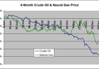
Summary Natural gas has slumped 33% over the last six months, but crude oil has fallen further, by 53%. As a result , the oil-gas ratio has tumbled 40% to 15.5, in the 4th percentile over the last five years. Theoretically, as gas becomes relatively more expensive to oil, drilling should shift away from oil and even into gas, if prices remain competitive, resulting in a normalization of the ratio. A long USO, short UNG pair trade will capitalize on this ratio returning to historical levels without net exposure to the tenuous commodity sector as a whole. Should the ratio return to its five year average of 25, a long USO/short UNG trade will net approximately 23%. A leveraged long UWTI/short UGAZ trade will yield approximately 70%. Investing in natural gas has been a challenge over the last year. After spiking to multi-year highs last winter thanks to the coldest winter in the past 20 years, the price of the commodity has been decimated over the past six months due to a combination of a mild summer and autumn that suppressed demand and record production. At Friday’s closing price of $3.12/MMBTU, the commodity is down 32.5% since June 1, 2014. As hard as it’s been to be a bull in the natural gas space, crude oil traders have an ever rougher deal. Thanks to record-setting U.S. production and OPEC willing to play a dangerous game of chicken with U.S. producers, the normally less-volatile crude oil is down 52.5% during the same period. Figure 1 below compares oil and natural gas prices over the last six months. (click to enlarge) Figure 1: 6-Month Oil/Gas Price Change (Pricing Data Sources EIA: NYMEX Futures Prices & Natural Gas Futures ) Depending on what source you read, oil is bound for either a rapid bounce to $60/barrel or doomed to slog around at $40/barrel for the next year or two. Likewise, for every article dooming natural gas to $2.00/MMBTU for the foreseeable future, another is predicting a new polar vortex that will send price soaring back to $4.00/MMBTU. Admittedly, there is an abnormally large degree of uncertainty in both sectors. Instead of trying to predict price movements in either commodity, this article will discuss a strategy to capitalize on a divergence from the historical relationship between the price of natural gas and oil. While natural gas has had a poor six-month performance, it is crude oil that has really been taken to the cleaners. As a result, natural gas has become more expensive relative to crude oil. Figure 2 below shows the Crude Oil-to-Natural Gas ratio over the last six years dating back to 2008. (click to enlarge) Figure 2: Oil-To-Gas Ratio 2008-Present (Source as above) The first half of 2008 marked the end of the era of vertical well drilling. In 2009 and beyond, directional drilling and fracking technology made the cost of hydrocarbon production significantly cheaper. However, the technology disproportionately benefited natural gas drillers. The crude oil-to-natural gas ratio therefore ballooned from around 12 in 2008 to a peak of 50 in early 2012 as natural gas prices plummeted to briefly under $2.00/MMBTU and oil prices stabilized around $100/barrel. The ratio has generally oscillated between 20 and 30 thereafter. However, as oil prices have tanked much faster than natural gas over the last six months, the ratio has plummeted over 40% from 27 in mid-July 2014 to 15.5 as of Friday’s close. This represents the 25th percentile since 2008 and the 4th percentile since 2010-the rough start of the fracking era. Rather than betting on a recovery in either natural gas or oil prices, an alternative strategy is a pair trade that bets on the recovery of this ratio to the historical range. This entails taking a short position in a natural gas ETF such as the United States Natural Gas ETF (NYSEARCA: UNG ) and a long position in an oil ETF such as the United States Oil ETF (NYSEARCA: USO ) such that a recovery in the crude oil-to-natural gas ratio will result in a net profitable position. If natural gas slumps and oil rallies-resulting in a rapid recovery in the ratio-both positions profit. If both natural gas and oil rally, but oil rallies more-resulting in a slower recovery in the ratio-the profits from the long oil position will outweigh the losses from the natural gas short. Likewise, should both fall but natural gas fall faster, the opposite will be true-profits from the natural gas short will outweigh losses from the oil long. Of course, should natural gas outperform oil, the pair trade will be a losing one-and because there is a short position involved, the losses may be extensive. However, this will result in the crude oil-to-natural gas ratio falling towards 10 and deviating even further from the historical averages. Approximate returns of this trade going long USO and short UNG are shown below in Figure 3 based on crude oil-to-natural gas ratio. I say “approximate” because the exact profitability varies slightly depending the exact prices of the two commodities (i.e. Oil at $60 and Gas at $3 vs. Oil at $40 and Gas at $2, both for a ratio of 20). These calculations assume a price of crude at $60/barrel, which represents the median of current analyst estimates for a 6 month price target, and natural gas at the corresponding value to satisfy the given ratio. Of note, real world returns may actually be boosted compared to these projections. It is well-established that rollover losses from contango can decimate an ETF. This is something that has plagued natural gas ETFs given the frequency at which this commodity trades with a large contango. Oil traditionally trades at a much smaller contango. Thus “excess” profits in the UNG short due to contango not affiliated with organic price movements will likely outweigh much smaller “excess” losses in the USO long due to contango. (click to enlarge) Figure 3: Projected profitability of a Long USO/Short UNG Pair Trade depending on Oil/Gas Ratio Should the ratio bounce just 30% to 20, the trade will return 14%. Should the ratio return to its 5-year historical average of 25, the trade returns 23%. I am currently invested in this trade using a position size that comprises 15% of my portfolio. Should the ratio slump under 15, I will look to slowly add to my positions. These returns can be boosted by using leveraged ETFs. Figure 4 below shows the same curve using a long Velocity Shares 3x Crude Oil ETN (NYSEARCA: UWTI ) and short Velocity Shares 3x Natural Gas ETN (NYSEARCA: UGAZ ) pair trade. (click to enlarge) Figure 4: Projected profitability of a Long UWTI/Short UGAZ Pair Trade depending on Oil/Gas Ratio Using this trade, profits will be around 41% should the ratio recover to 20 and 70% should the ratio climb to 25. However, this trade is not without risk. The excess leverage boosts losses such that should the crude oil-to-natural gas ratio fall to 10, losses will comprise the entire position due to the ballooning value of the short UGAZ short position. Secondly, the leveraged ETFs are not designed to track their underlying commodities in the long term. These ETFs tend to underperform, particularly in a choppy trade environment. Thus, should it take the oil-to-gas ratio > 6 months to reach a target level, expect actual returns to be less than projected. Beyond simple technicals-oil is due for a bounce after a nearly linear 6-month decline-the fundamental rational behind this trade is simple. As natural gas becomes more expensive relative to crude oil, it becomes less and less profitable to drill for liquid hydrocarbons versus gaseous hydrocarbons and rigs are gradually shunted from oil-directed to gas-directed. This trend is already reflected in the Baker Hughes Rig count. Figure 5 below shows the % change in oil-directed and gas-directed rigs over the past 6-months. (click to enlarge) Figure 5: Baker Hughes Rig Count Change In Oil And Gas Rigs Over The Last Six Months (Source: Baker Hughes ) Natural Gas-directed rigs have fallen 4.9% to 310 as of last Friday while Crude Oil rigs have fallen by 11.0% to 1366, or by 170 oil rigs and 16 gas rigs. Should this trend continue, it is likely that the crude oil supply will gradually stabilize while natural gas supply is more likely to remain near record levels, increasing the odds that the oil-to-gas ratio normalizes to historical levels. Additional disclosure: The author is also short UNG as discussed in the article.

And The Winner Is…

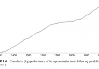
Until recently, the longest back test using stock market data was Geczy and Samonov’s 2012 study of relative strength momentum called “212 Years of Price Momentum: The World’s Longest Backtest: 1801-2012”. The length of that study has now been exceeded by an 800 year backtest of trend following absolute momentum in Greyserman and Kaminski’s new book, Trend Following with Managed Futures: The Search for Crisis Alpha . The authors looked at 84 equities, fixed income, commodities, and currencies markets as they became available from the years 1200 through 2013. They established long or short equal risk sized positions based on whether prices were above or below their 12-month rolling returns. The annual return of this strategy was 13% with an annual volatility of 11% and a Sharpe ratio of 1.16. Anyone who had doubts about the long-run efficacy of trend following momentum should no longer be doubtful. However, let’s not just look at trend following on its own. Let’s also compare it to other possible risk reducing or return enhancing approaches and see what looks best. We will base our comparisons on the performance of U.S. equities because that is where long-run risk premium and total return have been the highest. We also have U.S. stock market data available from the Kenneth French data library all the way back to July 1926. We will compare trend following to seasonality and then to the style and factor-based approaches of value, growth, large cap, and small cap. We will also see if it makes sense to combine these with trend following. For seasonality, we look at the Halloween effect, sometimes called “Sell in May and go away…” This has been known to practitioners for many years. There have also been a handful of academic papers documenting the positive results of holding U.S. stocks only from November through April. The following table shows the results of this strategy compared with absolute momentum applied to the broad U.S. stock market from May 1927 through December 2014. With 10-month absolute momentum, we are long stocks when the excess return (total return less the Treasury bill rate) over the past 10 months has been positive.[1] Otherwise, we hold Treasury bills. We also hold Treasury bills when we are out of U.S. stocks according to the Halloween effect (in stocks November-April, out of stocks May-October). We see that the 6-month seasonal filter of U.S. stock market returns substantially reduces volatility and maximum drawdown, but at the cost of reducing annual returns by over 200 basis points. Trend following absolute momentum, on the other hand, gives a greater reduction in maximum drawdown than seasonality with almost no reduction in return. There is no reason to consider seasonal filtering when absolute momentum gives a greater reduction in risk without diminished returns. The table below shows the U.S. market separated into the top and bottom 30% based on book-to-market (value/growth) and market capitalization (small/large). We see that value and small cap stocks have the highest returns but also the highest volatility and largest maximum drawdowns. Style US Mkt Value Growth Large Small Annual Return 11.8 16.2 11.3 11.5 16.6 Annual Std Dev 18.7 25.1 18.7 18.1 29.3 Annual Sharpe 0.42 0.46 0.39 0.42 0.41 Maximum DD -83.7 -88.2 -81.7 -82.9 -90.4 Most academic studies ignore tail risk/maximum drawdown, but these can be very important to investors. Not many would be comfortable with 90% drawdowns.[2] On a risk-adjusted basis (Sharpe ratio), neither small cap nor value stocks appear much better than growth or large cap stocks. This is consistent with the latest academic research showing no small size premium and a value premium associated only with micro cap stocks.[3] Let’s now see what happens now when we apply absolute momentum to these market style segments: Style w/Absolute Momentum AbsMom ValAbsMom GroAbsMom LgAbsMom SmAbsMom Annual Return 11.5 13.3 10.3 11.5 13.9 Annual Std Dev 12.9 17.2 13.3 12.5 21.1 Annual Sharpe 0.58 0.53 0.48 0.60 0.46 Maximum DD -41.4 -66.8 -42.3 -36.2 -76.9 In every case, adding absolute momentum reduces volatility, increases the Sharpe ratio, and substantially lowers maximum drawdown. The biggest impact of absolute momentum, however, is on large cap stocks, followed by the overall market index. The use of a trend following absolute momentum overlay further reduces the relative appeal of value or small cap stocks. We may wonder why large cap stocks respond better to trend following. The answer lies in a study by Lo and MacKinlay (1990) showing that portfolio returns are strongly positively autocorrelated (trend following), and that the returns of large cap stocks almost always lead the returns of small cap stocks. Since trend following lags behind turns in the market, investment results should be better if you can minimize that lag by being in the segment of the market that is most responsive to changes in trend. That segment is large cap stocks, notably the S&P 500 index, since they lead the rest of the market. In my book, Dual Momentum Investing: An Innovative Strategy for Higher Returns with Lower Risk , I give readers an easy-to-use, powerful strategy incorporating relative strength momentum to select between U.S. and non-U.S. stocks and absolute momentum to choose between stocks or bonds. I call this model Global Equities Momentum (GEM). And what index is the cornerstone of GEM? It’s the S&P 500, the one most responsive to trend following absolute momentum and that gives the best risk-adjusted results. Einstein said you should keep things as simple as possible, but no simpler. One can always create more complicated models or include more investable assets. But as we see here, trend following momentum is best when it is simply applied to large cap stocks. [1] We use 10-month absolute momentum instead of the more popular 10-month moving average because absolute momentum gives better results. See our last blog post, ” Absolute Momentum Revisited “. [2] The next largest maximum drawdown was 64.8 for value and 69.1 for small cap on a month-end basis. Intramonth drawdowns would have been higher. [3] See Israel and Moskowitz (2012) for empirical results. Delisting bias and high transaction costs can also reduce any small cap premium. Results are hypothetical, are NOT an indicator of future results, and do NOT represent returns that any investor actually attained. Indexes are unmanaged, do not reflect management or trading fees, and one cannot invest directly in an index. Please see our Disclaimer page for more information.

How To Design A Market Neutral Portfolio – Part 2

Summary Sector diversification is a key in market neutral investing. Two examples. Questions to solve for IRA compatibility. My previous article described the investor profile to hold a market neutral portfolio and some characteristics of this investing style illustrated by examples. I also explained why I prefer using an index ETF for the short side of the portfolio. In the next step, I want to focus on the benefit of sector diversification in market neutral investing. Sector diversification is especially important when the objective is to beat the benchmark in all market conditions, that is to say in all phases of the expansion-contraction cycle. The reality is more complicated than the figure. Cycles of different and variable periods may be in play, and macro trends can freeze the cycle for some sectors (like oil price does for energy and materials). In fact, it is sometimes quite difficult to figure out where we are and on which time frame when various cycles are combined. This is why, if an index ETF is on the short side, the long side of the portfolio must be diversified, not necessarily in all sectors, but at least in a few cyclical and defensive sectors. Since the return of such a Market Neutral Portfolio is the alpha of the long side, diversification in defensive and cyclical stocks is a key to keeping drawdowns acceptable in duration. In my opinion, the historical maximum duration in drawdown of an investing strategy is a parameter as important as the return and volatility. Examples I have performed a simulation of a portfolio mixing all the S&P 500 strategies of my book «The Lazy Fundamental Analyst» (Harriman House 2014). There are 9 strategies, one for each sector of the GICS classification, except Telecommunication (which is very small to elaborate statistical models). Each strategy selects 10 S&P 500 companies using a simple ranking process based on 2 fundamental factors. The factors are sector-dependent, chosen using historical statistics. The result is an equal-weighted portfolio of 90 stocks in a universe or 500, updated and rebalanced every 4 weeks. It is quite a big set (18% of the S&P 500 index) with various logics mixed, so the performance can hardly be suspected of being curve-fitted or random. Of course, past performance, real or simulated, is not a guarantee for future returns. But on such a portfolio it gives a good clue on the risk. The next chart shows the simulation of the 90-stock S&P 500 Lazy Portfolio (long side only) since 1999, with a 0.1% transaction cost and a 4-week rebalancing: (click to enlarge) The next table gives statistics of the excess return of the portfolio over the SPDR S&P 500 Trust ETF (NYSEARCA: SPY ) by 4-week periods, which corresponds to the market neutral portfolio with a leveraging factor 2, without the margin and carry cost for the “short half”. Average 4week return Average Annual return Max Drawdown Depth Max Drawdown Duration Avg gain / Avg loss 4week gain probability Kelly criterion Kelly crit. 95% confidence 0.94% 12.9% 20.5% 19 months 1.52 67% 0.46 0.35 Holding 90 stocks is a lot. In my real market neutral portfolio, I have reduced the number by: Excluding the most sensitive sectors to macroeconomic and geopolitical concerns: finance, energy and materials. My aim is not to get the best possible return, but a good return with a risk as low as possible. Optimizing the models to keep only 24 stocks with a diversification pattern, including at least 2 defensive sectors, 2 cyclical sectors and a minimum number of stocks in each of them. Optimizing to a lower number of stocks incurs a risk of curve fitting. However, with 24 holdings and various ranking logics, the risk remains quite low. The biggest danger of optimizing is not over-rating the possible return, but under-rating the real risk. In a diversified market neutral portfolio, the risk is limited by design. The next chart shows the simulation of my 24-stock portfolio (long side only) since 1999, with a 0.3% transaction cost and a 2-week rebalancing: (click to enlarge) This portfolio is more dynamic (rebalanced twice more often). It is also focused on large caps, but may hold a limited number of liquid small caps from the Russell 3000 index. Even if I use volume filters, I use a higher transaction cost to model a higher spread and slippage. The next table gives statistics of the excess return of the portfolio over SPY by 2-week periods, which corresponds to the market neutral portfolio leveraged twice, without the margin and carry cost. Average 2week return Average Annual return Max Drawdown Depth Max Drawdown Duration Avg gain/Avg loss 2week gain probability Kelly criterion Kelly crit. 95% confidence 0.79% 22% 11% 13 months 1.69 64.2% 0.43 0.36 These are examples. Ideas and steps can be reused with other quantitative models, or with a stock picking based on due diligence. The main idea here is to formalize and follow a sector-based diversification pattern. A next article will explain how to use leveraged ETFs to implement this strategy with a lower or no leverage (ProShares Ultra S&P 500 ETF (NYSEARCA: SSO ), ProShares UltraPro S&P 500 ETF (NYSEARCA: UPRO )), and the consequences of using inverse ETFs to avoid short selling (ProShares Short S&P 500 ETF (NYSEARCA: SH ), ProShares UltraShort S&P 500 ETF (NYSEARCA: SDS ), ProShares UltraPro Short S&P 500 ETF (NYSEARCA: SPXU )). Indeed market neutral investing can be implemented in an IRA account. Feel free to follow me if you don’t want to miss it. Data and charts: Portfolio123 Additional disclosure: Long SPXU as a hedge. Past performance is not a guarantee of future returns.