Tag Archives: author

How Cash Can Boost Long-Term Returns

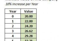
Summary Liquidity management is one of the most critical aspects of investment. Cash earns a 0% nominal return, but allows investors to take advantage of higher-return opportunities that may emerge. By holding more cash, one is betting that the purchasing power will increase at a future point. Moderation is key with holding cash; it’s rarely advisable to go to 100% cash or 0% cash. I’d recommend a cash position in the 20% – 40% range for most investors right now due to higher than average risks in the market. Buying stocks at depressed prices (i.e. with a large “margin of safety”) is the best way to generate superior returns over time. Cash, on the other hand, generates a 0% return. Absent a highly unlikely episode of hyper-deflation, you cannot become wealthy holding cash. In spite of this, I’d recommend holding 20% – 40% of your portfolio in cash right now. The reason for this is that there is value to liquidity, particularly in an inflated market environment. By holding cash, what you are actually doing is betting that the future value of your money in the market will be worth more than the present value. How can cash help you generate better returns? The key is to understand intrinsic value and the mathematics of investing. Intrinsic Value Price is what you pay for an asset. Intrinsic value is the fundamental worth of an asset. Therefore, an asset could be priced at $20,000, but have an intrinsic value of $30,000. In that instance, you are getting a bargain, because you are paying 33% less than the intrinsic value. In reality, it’s impossible to know the exact intrinsic value of a stock. None of us can see the future. Yet, we can come up with reasonable estimates of intrinsic value through a fundamental analysis of a company. That said, in order to explain why holding cash can be beneficial, we’ll first need to assume we can read the future. In this scenario, let’s say we know with absolute certainty that the intrinsic value of XYZ Company’s stock is $20. Now, we’re going to be able to live in five different alternate realities. In the first scenario, XYZ Company’s stock is selling at the depressed price of $5. In the second scenario, the stock sells at a still somewhat depressed price of $10. The third scenario will allow us to purchase the stock for $20; which is precisely the intrinsic value. In the fourth scenario the stock will sell at an inflated price of $25, and in the fifth scenario, it will sell at an even more inflated price of $30. Now, we’ll say that in each of our five alternate realities, we will purchase the stock and hold it for five years. We also know for a fact that the intrinsic value will grow 10% per year. You can see how the intrinsic value grows in the chart below. With that, let’s take a look at what happens. The Power of Compounding Now that we’ve created the set-up, you can see the return figures for all five scenarios below for a five-year holding period. It immediately becomes clear how dramatic the difference is between purchasing XYZ’s stock at a depressed price versus an inflated price. The “inflated price” only yields a 1.4% annual return, while the “depressed price” yields an astronomical 45.1% annual return! To put this further in perspective, if you started with $10,000 and generated a 45.1% annual return for the indefinite future, you would have $100,000 in a little over 6 years. On the other hand, if you generated a 1.4% for the foreseeable future, it would take you 166 years for you to turn that $10,000 into $100,000. That’s not a misprint! That’s the power of compounding. This is also the reason why an investor that generates a 17% annual return over 10 years is significantly better than one generating a 15% annual return. It may seem like a very small difference, but over a long-term timeframe, it really adds up. An investor making 15% annually on a $10,000 initial investment for 25 years would have $329,000 at the end of that timeframe. An investor generating a 17% annual return, on the other hand, would have $507,000; roughly 54% more. Why Cash is Valuable Given this math, it starts to become clearer why holding cash can sometimes led to higher long-term returns. Let’s say that XYZ’s stock was selling at the inflated price of $30, but you could see the future, and knew it could fall back down to $15 in 3 years. For simplicity’s sake, we’ll still assume that you plan to sell off at the end of Year #5 at the intrinsic value of $32.21. What would be your best option? (1) Buying the stock immediately and earning the 1.4% return for 5 years, (2) Holding cash for 3 years and then buying in at the semi-depressed price of $15 The answer is that option #2 is much more profitable. After five years, you’ll only generate a total return of 7.2% in Scenario #1, but you’ll achieve a 114.7% return in Scenario #2, in spite of the fact that you made a 0% return the first three years. This example showcases why the relationship between price and value are so important. It also shows why value investing works so well. What may seem like small differences in price can drive very large differences in return. Hold Some Cash Given the inflated market environment we are currently seeing, I believe it’s prudent to hold 20% – 40% of one’s portfolio right now. It’s true that you’ll likely underperform in the short-term (e.g. 1-3 years) as a result of this strategy. However, in the long-term, it makes more sense to take the 0% return now (on a part of your portfolio), and then use the liquidity to strike later when the returns become much more attractive. Of course, this should not dissuade you from taking advantage of bargains as you see them become available. And while I believe the broad market is overpriced, on a micro level, there will always be bargains out there. Yet, even if you can find a lot of bargains, I’d still recommend holding a good clip of cash, because even better bargains could become available the next time we find ourselves in a recession or a falling market environment. How much cash you hold in your portfolio depends upon your preferences and personal situation. If you’re in a situation where you can’t afford to lose much right now (i.e. you might need your cash for other purposes), I would recommend playing things fairly conservatively and holding a very large cash position. Even if you’re not worried about pulling out cash, I do think a minimum 10% cash position is prudent; and frankly, I wouldn’t dip below 20%. Conclusions Holding cash and generating a 0% return may seem like a poor option on the face of it, but once you understand the math behind returns, it makes a lot sense. By holding cash now, you’re hoping that you can generate higher returns in a future environment with lower prices. It’s never wise to go 100% cash, because at that point, you’re merely speculating. In an environment where stock prices seem inflated and there are few bargains out there, it makes sense to hold an elevated cash position in the range of 20% – 40% of your portfolio. On the other hand, in a depressed stock environment (such as the one we saw in late 2008 and early 2009), you should try to be as fully invested as possible, holding no more than 5% cash. Right now, I view us as being in an inflated environment and holding a 20% – 40% cash position is a prudent strategy. Your returns will lag in the short-term, but if there’s a market correction, you’ll more than make up for it in the long-term. This article appears in the February 2015 edition of Jake Huneycutt’s Contrarian Value Newsletter Disclosure: The author has no positions in any stocks mentioned, and no plans to initiate any positions within the next 72 hours. (More…) The author wrote this article themselves, and it expresses their own opinions. The author is not receiving compensation for it. The author has no business relationship with any company whose stock is mentioned in this article.

Investing For Retirement Using Northern Mutual Funds

Summary A set of just three Northern mutual funds, a bond, a large cap stock plus a mid cap fund generates good returns with relatively low risk. From January 2005 to January 2015, a Northern portfolio with fixed allocation could allow a safe 5% annual withdrawal rate with 1.36% increase of the capital. Same portfolio with rebalancing at 25% deviation from the target allowed a safe 5% annual withdrawal rate and 2.05% annual increase of the capital. Same portfolio with momentum-based adaptive allocation could have produced a safe 10% annual withdrawal rate and 1.26% annual increase of the capital. This article belongs to a series of articles dedicated for investing in various mutual fund families. In previous articles we reported our research on Fidelity , Vanguard , T Rowe Price , American Century , and Schwab mutual fund families. The current article does the same for Northern family of mutual funds. In addition, this article is the first in which a detailed study of the volatility of the returns using Sharpe and Sortino’s ratios is included. The series of these articles is aimed at a broad spectrum of investors. They may be useful to small individual investors as well as to any large institution managing retirement accounts. The general methodology we use in selecting the funds for the portfolio was presented in a previous article. The portfolio includes three funds: one bond fund and two equity funds. The equity funds are complementary: one covers large capitalization; the other fund contains medium capitalization stocks. The mutual funds selected for investment are the following: Northern us Treasury Index fund (MUTF: BTIAX ) Northern Stock Index fund (MUTF: NOSIX ) Northern Mid Cap Index fund (MUTF: NOMIX ) As in the previous articles, three different strategies are considered: (1) Fixed asset allocation. The portfolio is initially invested 50% in the bond fund and 50% equally divided between the two stock funds, without rebalancing. (2) Target asset allocation with rebalancing. The portfolio is initially invested 50% in the bond fund and 50% equally divided between the two stock funds and is rebalanced when the allocation to any fund deviates by 25% from its target. (3) Momentum-based adaptive asset allocation. The portfolio is at all times invested 100% in only one fund. The switching, if necessary, is done monthly at closing of the last trading day of the month. All money is invested in the fund with the highest return over the previous 3 months. The data for the study were downloaded from Yahoo Finance on the Historical Prices menu for three tickers: BTIAX, NOSIX, and NOMIX. We use the monthly price data from January 2005 to January 2015, adjusted for dividend payments. The paper is made up of two parts. In part I, we examine the performance of portfolios without any income withdrawal. In part II, we examine the performance of portfolios when income is extracted periodically from the accounts. Part I: Portfolios without withdrawals We report the performance of the portfolios under two scenarios: (1) no withdrawals are made during the time interval of the study, and (2) withdrawals at a fixed rate of the initial investment are made periodically. In table 1 we show the results of the portfolios managed for 10 years, from January 2005 to January 2015. Table 1. Portfolios without withdrawals 2005 – 2015. Strategy Total increase% CAGR% Number trades MaxDD% Fixed-no rebalance 93.45 6.82 0 -21.87 Target-25% rebalance 104.52 6.36 3 -31.09 Momentum-Adaptive 224.84 12.84 39 -13.35 In table 2 we show the results of a study on the volatility of the returns, including the much celebrated Sharpe and Sortino ratios. For completeness we give the definitions of these ratios. Sharpe ratio is the ratio of the compound annual growth rate (CAGR%) and the volatility of the returns (VOL%), where the volatility is defined as the annualized standard deviation of the returns. Sortino ratio is the ratio of the compound annual growth rate (CAGR%) and the volatility of the negative returns (NEG VOL%), where the volatility is defined as the annualized standard deviation of the negative returns. Table 2. Volatility performance of portfolios without withdrawals 2005 – 2015. Strategy CAGR% VOL% NEG VOL% Sharpe Sortino MaxDD% Fixed-no rebalance 6.82 7.18 6.29 0.95 1.08 -21.87 Target-25% rebalance 7.42 7.61 6.51 0.98 1.14 -31.09 Momentum-Adaptive 12.84 10.46 7.24 1.23 1.77 -13.35 By analyzing these results, one can see that the target portfolio has higher Sharpe and Sortino ratios than the fixed portfolio. On the other hand, the fixed portfolio has much lower maximum drawdown than the target portfolio. Which one is a better metric of risk: the volatility or the maximum drawdowns? Most investors, including the author of this article, are mostly concerned about large drawdowns, and pay less attention to Sharpe or Sortino ratios. The time evolution of the equity in the portfolios is shown in Figure 1. (click to enlarge) Figure 1. Equities of portfolios without withdrawals. Source: This chart is based on EXCEL calculations using the adjusted monthly closing share prices of securities. From figure 1 it is apparent that the rate of increase of the adaptive portfolio is substantially greater than the rate of the fixed and target allocation portfolios. Part II: Portfolios with withdrawals Assume that we invest $1,000,000 for income in retirement. We plan to withdraw monthly a fixed percentage of the initial investment. That amount is increased by 2% annually in order to account for inflation. In table 3 we show the results of the portfolios managed for 10 years, from January 2005 to January 2015. Money was withdrawn monthly at a 5% annual rate of the initial investment plus a 2% inflation adjustment. Over the 10 years from January 2005 to January 2015, a total of $535,920 was withdrawn. Table 3. Portfolios with 5% annual withdrawal rate 2005 – 2015. Strategy Total increase% CAGR% Number trades MaxDD% Fixed-no rebalance 14.51 1.36 0 -25.27 Target-25% rebalance 22.51 2.05 2 -26.77 Momentum-Adaptive 111.84 8.22 38 -16.56 The time evolution of the equity in the portfolios is shown in Figure 2. (click to enlarge) Figure 2. Equities of portfolios with 5% annual withdrawal rates. Source: This chart is based on EXCEL calculations using the adjusted monthly closing share prices of securities. To illustrate the advantage of the adaptive allocation strategy and the effect of withdrawal rates on the evolution of the capital, we give in Table 4 the results of simulations for the following withdrawal rates: 0%, 5%, 8%, and 10%. Table 4. Adaptive Portfolios with various annual withdrawal rates 2005 – 2015. Withdrawal rate % Total increase% CAGR% MaxDD% 0 224.84 12.84 -13.35 5 111.84 8.22 -13.97 8 52.33 4.53 -16.56 10 12.67 1.26 -20.25 The time evolution of the equity in the portfolios is shown in Figure 3. (click to enlarge) Figure 3. Equities of momentum-based portfolios with various annual withdrawal rates. Source: This chart is based on EXCEL calculations using the adjusted monthly closing share prices of securities. Conclusion The set of three Northern mutual funds, selected for this study, perform well for all three strategies and generate sustainable returns at relatively low drawdowns. Between 2005 and 2015, the fixed target allocation with rebalancing was able to sustain withdrawal rates of up to 5% annually. The adaptive allocation algorithm was able to sustain withdrawal rates up to 10% annually without any decrease of capital. Additional disclosure: This article is the sixth in a sequence on investing in mutual funds for retirement accounts. To help the reader compare the past performance of various mutual fund families, I selected a benchmark 10-year time interval starting on 1 January 2005 and ending on 31 December 2014. The article was written for educational purposes and should not be considered as specific investment advice. Disclosure: The author has no positions in any stocks mentioned, and no plans to initiate any positions within the next 72 hours. (More…) The author wrote this article themselves, and it expresses their own opinions. The author is not receiving compensation for it (other than from Seeking Alpha). The author has no business relationship with any company whose stock is mentioned in this article.

A New Event Debt ETF Filed By Eccles Street – ETF News And Commentary

A wide variety of products have been launched in the ETF world so far this year by several providers, big and small. Continuing this trend, Eccles Street Asset Management, which is a new player in the industry, looks to launch an active ETF targeting the fixed income ETF space. After all, every player is in a mad rush to tap the income/yields space, thanks to the global growth worries and the subsequent plunge in yields. The Proposed ETF in Focus Eccles Street Event Driven Opportunities ETF revolves around corporate bonds and bank loans having average portfolio duration of about 3-5 years, per the prospectus . Underlying securities will have maturity period within the same time range. The instruments are touted as “event-driven” as these revolve around corporate events. The Eccles Street Event Driven Opportunity ETF will also invest in equities, especially credit-related ETFs and ETNs. How Do These Fit in a Portfolio? The product could be an interesting choice for investors seeking a play in the bond market, which zeros in on high yielding securities. These products are for investors who wish to stay away from stock market volatility while at the same time seek a steady stream of cash flow from their portfolio. Moreover, these products also provide a big jump in yields as compared to treasuries when interest rates remain low. In the current environment, yield hungry investors view high yield corporate bonds as good sources to maximize current income in the form of interest, especially compared to other avenues which have low yields attached. Further, the short-to-intermediate span of the corporate bonds makes the ETF moderately interest-sensitive. With the Fed looking steadfast in its plan to raise the key rate this year, the shorter-end of the yield curve appears dicey. In such a backdrop, the intermediate-term bond ETFs might turn out as good picks. This is not the end though. The issuer is expected to choose less than investment grade securities, but the strengthening of corporate America should provide some cushion against default risks (read: 3 Ultra Safe Bond ETFs to Dodge Market Turmoil ). ETF Competition Peer pressure is presumably tough in the corporate bond ETF space. iShares iBoxx $ Investment Grade Corporate Bond Fund (NYSEARCA: LQD ) heads the space in terms of assets. The fund manages an asset base of over $20 billion, while charging investors just 15 basis points as fees. The fund has returned about 3% so far this year and has a yield of 3.03% (as of January 29, 2015) (read: Best and Worst Bond ETFs Of 2014 ). Another popular choice in the intermediate corporate bond ETF space that could be a threat to the newly filed product is iShares Intermediate Credit Bond ETF (NYSEARCA: CIU ) with an asset base of $6.36 billion. Yield-wise, SPDR Barclays Capital Long Term Corporate Bond ETF (NYSEARCA: LWC ) comes at the top producing 3.74% (as of January 29, 2015) (read: 3 Income ETFs to Watch if Rates Stay Low ). Thus, to garner enough investor confidence, the issuer needs to price its product competitively. The issuer also needs to watch that the yield factor – the main agenda of the product – is competitive.