Tag Archives: portfolios

Investing For Retirement Using Northern Mutual Funds

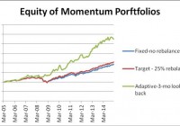
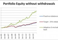
Summary A set of just three Northern mutual funds, a bond, a large cap stock plus a mid cap fund generates good returns with relatively low risk. From January 2005 to January 2015, a Northern portfolio with fixed allocation could allow a safe 5% annual withdrawal rate with 1.36% increase of the capital. Same portfolio with rebalancing at 25% deviation from the target allowed a safe 5% annual withdrawal rate and 2.05% annual increase of the capital. Same portfolio with momentum-based adaptive allocation could have produced a safe 10% annual withdrawal rate and 1.26% annual increase of the capital. This article belongs to a series of articles dedicated for investing in various mutual fund families. In previous articles we reported our research on Fidelity , Vanguard , T Rowe Price , American Century , and Schwab mutual fund families. The current article does the same for Northern family of mutual funds. In addition, this article is the first in which a detailed study of the volatility of the returns using Sharpe and Sortino’s ratios is included. The series of these articles is aimed at a broad spectrum of investors. They may be useful to small individual investors as well as to any large institution managing retirement accounts. The general methodology we use in selecting the funds for the portfolio was presented in a previous article. The portfolio includes three funds: one bond fund and two equity funds. The equity funds are complementary: one covers large capitalization; the other fund contains medium capitalization stocks. The mutual funds selected for investment are the following: Northern us Treasury Index fund (MUTF: BTIAX ) Northern Stock Index fund (MUTF: NOSIX ) Northern Mid Cap Index fund (MUTF: NOMIX ) As in the previous articles, three different strategies are considered: (1) Fixed asset allocation. The portfolio is initially invested 50% in the bond fund and 50% equally divided between the two stock funds, without rebalancing. (2) Target asset allocation with rebalancing. The portfolio is initially invested 50% in the bond fund and 50% equally divided between the two stock funds and is rebalanced when the allocation to any fund deviates by 25% from its target. (3) Momentum-based adaptive asset allocation. The portfolio is at all times invested 100% in only one fund. The switching, if necessary, is done monthly at closing of the last trading day of the month. All money is invested in the fund with the highest return over the previous 3 months. The data for the study were downloaded from Yahoo Finance on the Historical Prices menu for three tickers: BTIAX, NOSIX, and NOMIX. We use the monthly price data from January 2005 to January 2015, adjusted for dividend payments. The paper is made up of two parts. In part I, we examine the performance of portfolios without any income withdrawal. In part II, we examine the performance of portfolios when income is extracted periodically from the accounts. Part I: Portfolios without withdrawals We report the performance of the portfolios under two scenarios: (1) no withdrawals are made during the time interval of the study, and (2) withdrawals at a fixed rate of the initial investment are made periodically. In table 1 we show the results of the portfolios managed for 10 years, from January 2005 to January 2015. Table 1. Portfolios without withdrawals 2005 – 2015. Strategy Total increase% CAGR% Number trades MaxDD% Fixed-no rebalance 93.45 6.82 0 -21.87 Target-25% rebalance 104.52 6.36 3 -31.09 Momentum-Adaptive 224.84 12.84 39 -13.35 In table 2 we show the results of a study on the volatility of the returns, including the much celebrated Sharpe and Sortino ratios. For completeness we give the definitions of these ratios. Sharpe ratio is the ratio of the compound annual growth rate (CAGR%) and the volatility of the returns (VOL%), where the volatility is defined as the annualized standard deviation of the returns. Sortino ratio is the ratio of the compound annual growth rate (CAGR%) and the volatility of the negative returns (NEG VOL%), where the volatility is defined as the annualized standard deviation of the negative returns. Table 2. Volatility performance of portfolios without withdrawals 2005 – 2015. Strategy CAGR% VOL% NEG VOL% Sharpe Sortino MaxDD% Fixed-no rebalance 6.82 7.18 6.29 0.95 1.08 -21.87 Target-25% rebalance 7.42 7.61 6.51 0.98 1.14 -31.09 Momentum-Adaptive 12.84 10.46 7.24 1.23 1.77 -13.35 By analyzing these results, one can see that the target portfolio has higher Sharpe and Sortino ratios than the fixed portfolio. On the other hand, the fixed portfolio has much lower maximum drawdown than the target portfolio. Which one is a better metric of risk: the volatility or the maximum drawdowns? Most investors, including the author of this article, are mostly concerned about large drawdowns, and pay less attention to Sharpe or Sortino ratios. The time evolution of the equity in the portfolios is shown in Figure 1. (click to enlarge) Figure 1. Equities of portfolios without withdrawals. Source: This chart is based on EXCEL calculations using the adjusted monthly closing share prices of securities. From figure 1 it is apparent that the rate of increase of the adaptive portfolio is substantially greater than the rate of the fixed and target allocation portfolios. Part II: Portfolios with withdrawals Assume that we invest $1,000,000 for income in retirement. We plan to withdraw monthly a fixed percentage of the initial investment. That amount is increased by 2% annually in order to account for inflation. In table 3 we show the results of the portfolios managed for 10 years, from January 2005 to January 2015. Money was withdrawn monthly at a 5% annual rate of the initial investment plus a 2% inflation adjustment. Over the 10 years from January 2005 to January 2015, a total of $535,920 was withdrawn. Table 3. Portfolios with 5% annual withdrawal rate 2005 – 2015. Strategy Total increase% CAGR% Number trades MaxDD% Fixed-no rebalance 14.51 1.36 0 -25.27 Target-25% rebalance 22.51 2.05 2 -26.77 Momentum-Adaptive 111.84 8.22 38 -16.56 The time evolution of the equity in the portfolios is shown in Figure 2. (click to enlarge) Figure 2. Equities of portfolios with 5% annual withdrawal rates. Source: This chart is based on EXCEL calculations using the adjusted monthly closing share prices of securities. To illustrate the advantage of the adaptive allocation strategy and the effect of withdrawal rates on the evolution of the capital, we give in Table 4 the results of simulations for the following withdrawal rates: 0%, 5%, 8%, and 10%. Table 4. Adaptive Portfolios with various annual withdrawal rates 2005 – 2015. Withdrawal rate % Total increase% CAGR% MaxDD% 0 224.84 12.84 -13.35 5 111.84 8.22 -13.97 8 52.33 4.53 -16.56 10 12.67 1.26 -20.25 The time evolution of the equity in the portfolios is shown in Figure 3. (click to enlarge) Figure 3. Equities of momentum-based portfolios with various annual withdrawal rates. Source: This chart is based on EXCEL calculations using the adjusted monthly closing share prices of securities. Conclusion The set of three Northern mutual funds, selected for this study, perform well for all three strategies and generate sustainable returns at relatively low drawdowns. Between 2005 and 2015, the fixed target allocation with rebalancing was able to sustain withdrawal rates of up to 5% annually. The adaptive allocation algorithm was able to sustain withdrawal rates up to 10% annually without any decrease of capital. Additional disclosure: This article is the sixth in a sequence on investing in mutual funds for retirement accounts. To help the reader compare the past performance of various mutual fund families, I selected a benchmark 10-year time interval starting on 1 January 2005 and ending on 31 December 2014. The article was written for educational purposes and should not be considered as specific investment advice. Disclosure: The author has no positions in any stocks mentioned, and no plans to initiate any positions within the next 72 hours. (More…) The author wrote this article themselves, and it expresses their own opinions. The author is not receiving compensation for it (other than from Seeking Alpha). The author has no business relationship with any company whose stock is mentioned in this article.

Investing For Retirement Using American Century Mutual Funds

Summary American Century offers a set of diversified mutual funds which can be successfully used for construction of investment portfolios with good withdrawal rates. A set of just three mutual funds, a bond, an equity growth, plus an equity value fund generates good returns with relatively low risk. From January 2005 to December 2014, an American Century portfolio with fixed allocation could produce a safe 5% annual withdrawal rate and 2.15% annual increase of the capital. Same portfolio with rebalancing at 25% deviation from the target allowed a safe 5% annual withdrawal rate and achieved 2.21% compound annual increase of the capital. Same portfolio with momentum-based adaptive allocation could have produced a safe 12% annual withdrawal rate and 3.51% annual increase of the capital. This article belongs to a series of articles dedicated for investing in various mutual fund families. In previous articles we reported our research on Fidelity , Vanguard , and T Rowe Price mutual fund families. The current article does the same for American Century family of mutual funds. The series of these articles is aimed at a broad spectrum of investors. They may be useful to small individual investors as well as to any large institution managing retirement accounts. We report the performance of the portfolios under two scenarios: (1) no withdrawals are made during the time interval of the study, and (2) withdrawals at a fixed rate of the initial investment are made periodically. Since this is the fourth family of mutual funds for which we are building an investment portfolio for retirement, we elaborate here upon the general methodology we use. The set of funds selected for building the portfolio should satisfy the following criteria: (1) It should include at least one bond fund. (2) It should include a few equity funds, generally between two to five. Those funds should have enough similarity and diversity. As an example, we may select one value and one growth fund. (3) Historically, the funds selected should have performed better than most other funds in their category. Applying these principles, we selected three mutual funds for inclusion in a portfolio of American Century mutual funds. They are the following: American Century Government bond fund (MUTF: CPTNX ) American Century Heritage fund (MUTF: TWHIX ) American Century Value fund (MUTF: TWVLX ) As in the previous articles, three different strategies are considered: (1) Fixed asset allocation. The portfolio is initially invested 50% in the bond fund and 50% equally divided between the two stock funds, without rebalancing. (2) Target asset allocation with rebalancing. The portfolio is initially invested 50% in the bond fund and 50% equally divided between the two stock funds and is rebalanced when the allocation to any fund deviates by 25% from its target. (3) Momentum-based adaptive asset allocation. The portfolio is at all times invested 100% in only one fund. The switching, if necessary, is done monthly at closing of the last trading day of the month. All money is invested in the fund with the highest return over the previous 3 months. The data for the study were downloaded from Yahoo Finance on the Historical Prices menu for three tickers: CPTNX, TWHIX, and TWVLX. We use the monthly price data from January 2005 to December 2014, adjusted for dividend payments. The paper is made up of two parts. In part I, we examine the performance of portfolios without any income withdrawal. In part II, we examine the performance of portfolios when income is extracted periodically from the accounts. Part I: Portfolios without withdrawals In table 1 we show the results of the portfolios managed for 10 years, from January 2005 to December 2014. Table 1. Portfolios without withdrawals 2005 – 2014. Strategy Total increase% CAGR% Number trades MaxDD% Fixed-no rebalance 103.55 7.30 0 -24.61 Target-25% rebalance 109.82 7.63 4 -22.03 Momentum-Adaptive 330.90 15.73 35 -13.97 The time evolution of the equity in the portfolios is shown in Figure 1. (click to enlarge) Figure 1. Equities of portfolios without withdrawals. Source: This chart is based on EXCEL calculations using the adjusted monthly closing share prices of securities. From figure 1 it is apparent that the rate of increase of the adaptive portfolio is substantially greater than the rate of the fixed and target allocation portfolios. Part II: Portfolios with withdrawals Assume that we invest $1,000,000 for income in retirement. We plan to withdraw monthly a fixed percentage of the initial investment. That amount is increased by 2% annually in order to account for inflation. In table 2 we show the results of the portfolios managed for 10 years, from January 2005 to December 2014. Money was withdrawn monthly at a 5% annual rate of the initial investment plus a 2% inflation adjustment. Over the 10 years from January 2005 to December 2014, a total of $535,920 was withdrawn. Table 2. Portfolios with 5% annual withdrawal rate 2005 – 2014. Strategy Total increase% CAGR% Number trades MaxDD% Fixed-no rebalance 24.03 2.15 0 -28.78 Target-25% rebalance 22.68 2.21 4 -27.04 Momentum-Adaptive 210.05 11.98 35 -16.41 The time evolution of the equity in the portfolios is shown in Figure 2. (click to enlarge) Figure 2. Equities of portfolios with 5% annual withdrawal rates. Source: This chart is based on EXCEL calculations using the adjusted monthly closing share prices of securities. To illustrate the effect of the withdrawal rates on the evolution of the capital we report simulation results for two strategies: fixed target with rebalancing and momentum-based adaptive asset allocation. In Table 3 we report the results of simulations of the fixed target portfolio with the following withdrawal rates: 0%, 5%, 6%, 8%, and 10%. The time evolution of the equity in the portfolios is shown in Figure 3. To illustrate the advantage of the adaptive allocation strategy and the effect of withdrawal rates on the evolution of the capital, we give in Table 3 the results of simulations for the following withdrawal rates: 0%, 5%, 10%, and 12%. Table 3. Adaptive Portfolios with various annual withdrawal rates 2005 – 2014. Withdrawal rate % Total increase% CAGR% MaxDD% 0 330.90 15.73 -13.97 5 210.05 11.98 -16.41 10 89.54 6.60 -20.24 12 41.20 3.51 -22.23 The time evolution of the equity in the portfolios is shown in Figure 3. (click to enlarge) Figure 3. Equities of momentum-based portfolios with various annual withdrawal rates. Source: This chart is based on EXCEL calculations using the adjusted monthly closing share prices of securities. Conclusion The set of three American Century mutual funds, selected for this study, perform well for all three strategies and generate sustainable returns at relatively low drawdowns. Between 2005 and 2015, the fixed target allocation with rebalancing was able to sustain withdrawal rates of up to 6% annually. The adaptive allocation algorithm was able to sustain withdrawal rates up to 13% annually without any decrease of capital. We must admit here that the performance of the portfolio selected in this article is by no means the best possible. Without doubt, there may be other selections that would have performed better. On the other hand, past performance does not guarantee future results. Finding the best portfolio even for a specified past time interval is a great undertaking. All we can do is to strive toward finding one of the best, not really the best. Same philosophy applies into selecting the family of funds. In an article at the end of the series we will present a comparative study of their relative performance. Disclosure: The author has no positions in any stocks mentioned, and no plans to initiate any positions within the next 72 hours. (More…) The author wrote this article themselves, and it expresses their own opinions. The author is not receiving compensation for it (other than from Seeking Alpha). The author has no business relationship with any company whose stock is mentioned in this article. Additional disclosure: This article is the fourth in a sequence on investing in mutual funds for retirement accounts. To help the reader compare the past performance of various mutual fund families, I selected a benchmark 10-year time interval starting on 1 January 2005 and ending on 31 December 2014. The article was written for educational purposes and should not be considered as specific investment advice.

What To Do About Poor Future Returns

There’s been a lot of chatter recently about asset valuations, in particular U.S. stocks and U.S. bonds, and their impact of future returns. This is nothing new. It just seems to get louder at the start of every new year. I’ve discussed this topic before on the blog. Last time here . Basically, my point was that we may indeed, in fact it’s probable, be facing poor future returns – a least for the next 10 years, but that doesn’t mean that the 4% SWR rule is dead. In fact the 4% SWR implies even worse returns than people are forecasting now. For those building towards retirement it probably means a longer time to hit one’s goals And maybe that’s the worst part of it. In this post I wanted to discuss what the options are for investors if we take the forecasts of poor future returns as a fait accompli. First, some discussion of definitions is in order. Most of the the time when you hear forecasts of poor future returns you hear about the potential for poor U.S. stock returns, and poor U.S. government bonds returns, and the predominant 60% U.S. stock 40% U.S. bond allocation. The 60/40 portfolio is the dominant benchmark used in the U.S. by the finance industry partially due to the fact that they are the asset classes with the best and longest historical data. That is why you hear about it so much. Part of the problem with this of course is that today there are far more assets classes than just these basic two. But for this type of analysis it serves the purpose well enough. Just something to be aware of. Let’s move on. In this post, I’m going to use a recent forecast analysis done by Research Affiliates at the beginning of the year that forecasts future 10yr real asset class returns and the 60/40 portfolio return. You can find that analysis here . They also maintain an updated forecast of 10 yr expected real returns at their asset allocation website . A must visit in my view. Here is a graphical view of their current 10 yr real return forecasts and risk. The classic 60/40 portfolio is way down there. Almost at the bottom left corner with a 10 yr projected real return of 0.4% annualized. Not so great. They forecast U.S. large stocks at 0.4% as well, so that basically leaves 0.4% for bond returns, the benefits of re-balancing, etc. Not exactly outstanding. Just for reference, over the last 10 year period from 2005 to 2014, the 60/40 portfolio has returned 4.8% per year on a real basis, not too far from it’s historical average of 5.2% per year. Let’s take these forecasts as a given and discuss what options an investor has going forward. The most obvious option is to do nothing. If these forecasted returns do come to represent reality then, at least for those withdrawing from their portfolios, the historical 4% SWR will probably be just fine. As the Kitces blog post I linked to in the first paragraph discusses in detail these forecasts of poor future returns would turn out to be an upside surprise to the 4% SWR. In fact, for the worst case retiree in history, starting in 1966, the first 10 year return for a 60/40 portfolio was -1.85% real per year! That’s a lot lower than what is currently being forecasted. In the modern portfolio era, since 1973, there have been four 10 yr periods where the real return was less than 1% per year. Those were the 10 yr periods beginning in 1973, 1999, 2000, and 2001. Sometimes you get the impression that the realization of these poor forecasted returns would be some unprecedented event. Not even close. We’ve been there before and in not the too distant past either. A slight variation to the do nothing option is just to change the allocation between stocks and bonds. If stocks are not offering any higher real returns than bonds then why allocate to them. For example, an investor could go to a 40% stock 60% bond allocation (or 50/50, 30/70, etc…), that has the same forecasted real return but with a lot lower volatility and lower drawdowns. The lower volatility and drawdowns in and of themselves will lead to higher SWRs. The next option is to allocate to assets classes with higher forecasted returns. Obvious, right? The tough part is deciding how to break up that allocation and to into what asset classes. It is much better to simply choose a long standing portfolio allocation that has stood the test of time. I’ll use two examples here that I talk about often on the blog; the Permanent Portfolio, and the IVY 5 asset class buy and hold portfolio. Taking the asset allocations for the portfolios and plugging in the forecasted returns from the Research Affiliates forecast you get the forecasted 10yr returns for the strategies shown below. The Permanent Portfolio’s forecasted 10 yr real return is 0.9%. That’s much better than 60/40 but still a lot less than it’s average 10yr real return since 1973 of 5%. However the Permanent Portfolio comes with a lot less volatility (30% less) than 60/40 and a lot lower drawdowns which leads to a higher SWR than implied just by the return alone. The IVY5 Portfolio’s forecasted 10 yr real return is 2.2%, compared with it’s 7% average since 1973. I didn’t forecast the IVY13 portfolio because there were no forecasts for certain key factors, like value and momentum, but assuming historical relationships, lets say the IVY13 forecasted 10yr real returns are in the 2.5% to 3% per year. As you can see, going global and diversifying more enhances the projected returns. Now, lets see how some of the tactical asset allocation models may perform in the future under these poor future return forecasts. For this part of the discussion, I’ll be comparing the GTAA5, GTAA13, GTAA AGG3, and GTAA AGG6 portfolios to the buy and hold portfolios discussed above. The first thing I’ll do is compare the performance of the tactical asset allocation portfolios over all 10 yr periods to the buy and hold portfolios; 60/40, IVY5, and Permanent. Then we’ll compare the performance over only the worst 10 yr periods. That will give us a gauge of their relative performance during these bad return periods we are interested in. Below is the key table. The first line in the table shows the average real 10 yr period performance for each of the portfolios for all 10 yr periods since 1973 (1973 to 1982, 1974 to 1983…through 2005 to 2014). The 60/40 portfolio returned on average 5.82% real per year, the IVY5 7.06%, the AGG6 portfolio 14.15%, etc… The next row shows the spread between the particular portfolio and the 60/40 classic buy and hold portfolio. For example, GTAA5 outperforms 60/40 on average about 1.82% per year. Now it gets interesting. The next row shows the average 10 yr period performance only for those 10 yr periods where the 60/40 return was less than 1% per year real. The performance for all the portfolios is lower as one would expect but look at the next row, the spreads to the 60/40 portfolio during these poor return periods. The outperformance of all the portfolios is better during bad periods. For example, GTAA5 only outperforms 60/40 by 1.82% per year during all periods but during bad periods it outperforms by 6.8% per year! That is pretty astonishing. The TAA portfolios have risk reduction built in automatically and keep the investor out of long down markets, exactly what is being forecasted for the buy and hold portfolios. Sounds like a pretty good portfolio approach to me especially if the forecast of poor returns comes to be. If similar spreads hold true in the future the TAA portfolios would be looking at 10 yr real performance ranges of 6-8% per year for the GTAA5 and GTAA13 portfolios and 13-15% per year for the GTAA AGG3 and AGG6 portfolios. Sounds to good to be true but even if the performance ranges are half of what they’ve been an investor will be a lot better off than in a traditional 60/40 portfolio. The structure of the portfolios stacks the odds in the investor’s favor during bad markets. In summary, I’ve shown that if forecasts of poor returns come true the portfolio outcomes for investors are no worse than the past. An investor doesn’t need to do anything different. But there are better options that stack the odds in the investor’s favor in poor return environments. The most basic option is better diversification as exhibited in the IVY5 and the Permanent Portfolio as examples. And then there are even better options by using tactical allocation models that protect to the downside and in aggressive versions tilt the portfolio toward the best performing asset classes. While all returns for all portfolios will be lower in a low return environment the outperformance of better constructed portfolios will still allow investors and especially retirees to outperform and meet their long term goals.