Tag Archives: alt-investing

The Low Volatility Anomaly: Mid Caps

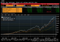
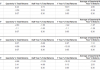
The Low Volatility Anomaly describes portfolios of lower volatility securities that have produced higher risk-adjusted returns than higher volatility securities historically. This article provides additional evidence for Low Volatility strategies by showing the factor’s success in mid-cap stocks. Provides historical comparison of returns between low volatility mid cap stocks versus broad mid cap indices and the benchmark large cap index. Thus far in this series, our most oft used description of the Low Volatility Anomaly in equity markets has been depicted through the use of a factor tilt on a large cap index. In the introductory article to this series on Low Volatility Investing, I plotted the cumulative total return profile (including reinvested dividends) of the S&P 500 (NYSEARCA: SPY ), the S&P 500 Low Volatility Index (NYSEARCA: SPLV ), and the S&P 500 High Beta Index (NYSEARCA: SPHB ) over the past twenty-five years. In an article last week , I showed that the Low Volatility Anomaly extends to small cap stocks as well as the S&P Smallcap 600 Low Volatility Index has also outperformed the broader S&P Smallcap 600 over the last twenty years, producing annual total returns of nearly 14% per annum. The volatility-tilted indices for both the small and large cap indices are comprised of the twenty percent of index constituents with the lowest (highest) volatility within the S&P 500 based on daily price variability over the trailing one year, rebalanced quarterly, and weighted by inverse (direct) volatility. The low volatility tilt of both the small and large cap indices produced both higher absolute returns and much lower variability of returns than the broader market gauges. This article will answer the question of whether such a factor tilt delivers alpha in the space in-between – the mid-cap stock market. Fortunately for our examination, Standard & Poor’s has also developed the S&P MidCap 400 Low Volatility Index . Similar to the S&P 500 Low Volatility Index, this benchmark tracks the twenty percent of the S&P MidCap 400 (eighty stocks) with the lowest realized volatility over the past year, weighted by an inverse of that volatility, and then rebalanced quarterly. While the index was launched in September 2012, Standard & Poor’s has back-tested data for over twenty years. Below is a graph of the cumulative total return of the S&P MidCap 400 Low Volatility Index, the S&P MidCap 400 Index, and the S&P 500. (click to enlarge) Source: Standard and Poor’s; Bloomberg As you can see above, the S&P MidCap 400 Index (white line; replicated through the ETF MDY ) readily bests the S&P 500 (yellow line). This outperformance is consistent with my article on 5 Ways to Beat the Market that demonstrated the structural alpha available through the size factor, which has been well documented in academic research (F ama & French, 1992 ). Some readers have also contended that the outperformance from Equal Weighting, which was also one of my “5 Ways ” is attributable to the size factor as well and more reminiscent of a mid-cap strategy given the lower average capitalization of equally weighting versus traditional capitalization weighting, but I contend that the contrarian re-balancing also contributes to the alpha-generative nature of that strategy. Whatever the source of the structural alpha, mid-caps have outperformed large-caps over long-time intervals. Low Volatility mid-caps have outperformed the broad mid-cap index on a risk-adjusted basis, but not on an absolute basis like the Small and Large Cap strategies. In tabular form, one can readily see that each of the small cap, mid cap, and large cap Low Volatility indices produce higher risk-adjusted returns with lower variability of returns than the broader market gauges from which they are constructed. The lower downside in the market selloff in 2008 greatly contributes to the lower variability of the Low Volatility indices. (click to enlarge) The PowerShares S&P MidCap Low Volatility Portfolio (NYSEARCA: XMLV ) seeks to replicate the performance of the S&P MidCap 400 Low Volatility Index with a 0.25% expense ratio. Like many of the Low Volatility ETFs, XMLV is a post-crisis innovation with a track record dating only back to February 2013. The ETF has only $100M of AUM, and thirty-day average volume of only 14,600 shares, similar AUM to the SmallCap Low Volatility ETF (NYSEARCA: XSLV ), but about 2/3 of the trading volume. Again similar to the Small Cap Low Volatility Index, I would be remiss if I did not mention that financials currently account for nearly half of the fund weighting (REITs 27.3%, Insurance 16.6%, Banks 3.8%). As I covered in a recent comparison between the PowerShares S&P Low Volatility ETF versus the iShares MSCI USA Minimum Volatility ETF (NYSEARCA: USMV ), industry concentrations in the S&P indices are uncapped, unlike the MSCI versions, and this lack of constraints has historically led to risk-adjusted outperformance and more variable industry concentrations over time. A reader of my article on Small Cap Low Volatility contended that they disfavored these funds because of the potential higher sensitivity to higher rates given the financial bent. Rates are moderately higher in 2015, and XMLV has delivered market-beating returns. I would point out that if higher rates lead to higher return volatility, then these stocks will be attributed lower weights or excluded from the fund at the quarterly rebalance date. As described in now fourteen recent articles on the Low Volatility Anomaly, I am a believer in the relative risk-adjusted outperformance of low volatility strategies. While Mid-Cap Low Volatility did not deliver the absolute outperformance versus the Mid Cap Index over the historical sample period, it still strongly outpeformed on a risk-adjusted basis. Versus the S&P 500, which many use as their benchmark, MidCap Low Volatility still delivered 3% per annum of outperformance with less than three-quarters of the return volatility. I am also a believer in the long-run outperformance available through the size factor that favors smaller and mid-capitalization stocks. Resultantly, I am evaluating an entry into a modest position to XMLV to provide some additional diversification to the Low Volatility portion of my long-term portfolio and will monitor the efficacy of this ETF vehicle as it matures. Disclaimer: My articles may contain statements and projections that are forward-looking in nature, and therefore inherently subject to numerous risks, uncertainties and assumptions. While my articles focus on generating long-term risk-adjusted returns, investment decisions necessarily involve the risk of loss of principal. Individual investor circumstances vary significantly, and information gleaned from my articles should be applied to your own unique investment situation, objectives, risk tolerance, and investment horizon Disclosure: I am/we are long SPY, SPLV, XSLV. (More…) I wrote this article myself, and it expresses my own opinions. I am not receiving compensation for it (other than from Seeking Alpha). I have no business relationship with any company whose stock is mentioned in this article.

Tactical Asset Allocation – My Ideas From 30 Years Of Learning

Summary How to create an investment portfolio using Tactical Asset Allocation. Three key measures I use are interest rates, valuation, and growth outlook. When selecting countries or regions, consider demographics, job growth, urbanization, debt levels, geo-political risk and currency effects. Tactical Asset Allocation (TAA) is defined as a dynamic investment strategy that actively adjusts a portfolio’s asset allocation . My goal in this article is to share with you the ideas that I have developed over the past 30 years, and to encourage discussion amongst readers, so as we can all learn from each other’s ideas and experiences. Introduction As a financial adviser, I must first consider a client’s risk profile. Younger clients with less capital invested will typically be prepared to take on more risk, and older clients will usually be comfortable taking on less risk. To keep it simple, I consider the following four asset classes: Cash, Bonds (CDs), Property and Equities. NB: I may also add Infrastructure (when interest rates are low to medium) or other sector funds, on occasion, as a small percentage of the portfolio. In determining my clients’ asset allocation, I consider the following factors: Interest rates Valuation Growth outlook Interest Rates The table below guides me, as does the 10-year Bond rate versus the equities dividend yield. BEST WORST Interest Rates Number 1 Number 2 Number 3 Number 4 Low (0-3%) Property Equities Bonds (CDs) Cash Medium (3-6%) High (6%+) Cash Bonds (CDs) Equities Property NB: The above % interest rates above are based on the reserve bank rate. Typically, the actual lending rates are around 2-3% higher. NB: When interest rates are “Medium” (3-6%), then their effect on the four asset classes is fairly neutral. Interest rates falling is better for bonds (CDs), property and equities. Interest rates rising is better for cash. Valuation My preferred valuation measures for asset allocation are: Price Earnings (P/E) Ratio : I look at a region or country’s P/E, both historical (last year’s earnings) and forward P/E, where available. My rule of thumb is to buy heavily as the P/E heads towards 10 and sell heavily as the P/E heads towards 20. A P/E of 15 is considered neutral. Having said that, I will also factor in interest rates. The Rule of 20 holds that P/E should be 20 minus the current interest rate. E.g., USA’s P/E should currently be 20 – 0.25 = 19.75. This makes allowance for times of extreme interest rates, as does the table below on interest rates. Long-term Charts of a Country’s Equity Index : Here, I simply view a 10- or 20-year chart and see if the index is above or below its trend line. Above being overvalued, below undervalued. Growth Outlook I will assess the following for a region’s or country’s growth outlook; GDP – Current year and forecast for next year. Earnings Per Share (EPS) – Forecast for next year. I will take a look at the following factors: Demographics – Is there a rising middle class, a growing work force or wealth effect? (You can read my article on demographics here , and the one on the rising Asian middle class here .) Job growth (unemployment) – Is the country gaining jobs? Urbanization – Is the country urbanizing? Debt levels – Are household debt levels low? Geopolitical risk and quality of government – Is there low geopolitical risk? Currency valuation – Is the currency undervalued? Trying to factor in all of the above is, of course, no easy task. Nor is it an exact science, but rather, is an art form, in my opinion. Having said that, I will give an example below of how I am currently (as of August 2015) recommending to my Australian clients, based on the above. Moderate-Risk Australian Client – $1m (AUD) Cash – 30% Bonds (Term Deposits, or TDs) – 0% Property – 20% Equities (comprising Asia) – 40% Sector funds – 10% (comprising Global Infrastructure – 5%, Global Resources – 5%) NB: TDs in Australia are the same as CDs in USA. Discussion on the above Tactical Asset Allocation Cash – 30% : Low percentage, as aggressive client and interest rates are very low. The reason to maintain 30% is to have cash available (to protect and invest) in case we see a severe market correction. Cash rates in Australia are still around 2.5% p.a. Bonds – 0% : Zero percentage, as interest rates are falling in Australia. 0% to International bonds, as the rates are already very low in developed markets. Could consider Asian or emerging market bond funds, where the rates are around 5-6% p.a., but there would be currency risk. Property – 10% in Australian-listed property : Low percentage due to earnings growth outlook being weak, with a weak Australian economy and rising unemployment. Low interest rates and fair valuation (P/E 15) suggest some exposure is necessary. Finally, most Australians already have very large $ exposure to an overvalued residential property sector. 10% in Global-listed property : Low interest rates are favourable and valuations fair. Equities – 40% : High percentage due to low interest rates, fair valuations in some regions/countries, strong growth prospects in Asia (demographics mostly good, rising middle class set to triple in size by 2020, according to DBS , with good jobs growth, urbanization, mostly low household and government debt levels, mostly low geo-political risk, and mostly good governments). Global Infrastructure – 5% : Low due to valuations being somewhat elevated. Could go to 10%, based on low global interest rates. Global Resources – 5% : Low, as this sector has been smashed down, and Asian demand for resources will pick up, with 290 million new homes required by 2020 and massive infrastructure projects planned. The valuations may look a bit high, but they are based on very low commodity prices at present. The following P/Es and growth outlook were part of the consideration. Australia: P/E – 15.67, Growth outlook – Poor Asia: P/E – 17.05, Growth outlook – Strong USA: P/E – 19.92, Growth outlook – Average-to-poor Europe: P/E – 19.11, Growth outlook – Average-to-poor Japan: P/E – 16.91, Growth outlook – Average-to-poor The above allocations will certainly lead to many debates, and this is healthy. US investors will naturally have more exposure to their local assets, which will avoid currency risk. They may choose to hold a percentage in US shares, given that the long-term outlook for US companies is strong. I do not disagree with that. My concerns are for non-US investors buying into the US late in the bull run, with a high valuation and a high USD. The main point of this article is to give investors some ideas on how they can go about building their portfolios, with consideration to both risk and return. For me, as discussed, I like to start with interest rates, then consider valuations and growth outlook. I always keep one eye on risk control and the other on optimizing returns, based on the client’s risk tolerance. Disclosure: I/we have no positions in any stocks mentioned, and no plans to initiate any positions within the next 72 hours. (More…) I wrote this article myself, and it expresses my own opinions. I am not receiving compensation for it (other than from Seeking Alpha). I have no business relationship with any company whose stock is mentioned in this article. Additional disclosure: The information in this article should not be relied upon as personal advice.

Dual Momentum August Update

Scott’s Investments provides a free “Dual ETF Momentum” spreadsheet, which was originally created in February 2013. The strategy was inspired by a paper written by Gary Antonacci and available on Optimal Momentum . Antonacci’s book, ” Dual Momentum Investing: An Innovative Strategy for Higher Returns with Lower Risk “, also details Dual Momentum as a total portfolio strategy. My Dual ETF Momentum spreadsheet is available here , and the objective is to track four pairs of ETFs and provide an “Invested” signal for the ETF in each pair with the highest relative momentum. Invested signals also require positive absolute momentum, hence the term “Dual Momentum”. Relative momentum is gauged by the 12-month total returns of each ETF. The 12-month total returns of each ETF is also compared to a short-term Treasury ETF (a “cash” filter) in the form of the iShares Barclays 1-3 Year Treasury Bond ETF (NYSEARCA: SHY ). In order to have an “Invested” signal, the ETF with the highest relative strength must also have 12-month total returns greater than the 12-month total returns of SHY. This is the absolute momentum filter, which is detailed in depth by Antonacci, and has historically helped increase risk-adjusted returns. An “average” return signal for each ETF is also available on the spreadsheet. The concept is the same as the 12-month relative momentum. However, the “average” return signal uses the average of the past 3-, 6-, and 12- (“3/6/12”) month total returns for each ETF. The “invested” signal is based on the ETF with the highest relative momentum for the past 3, 6 and 12 months. The ETF with the highest average relative strength must also have an average 3/6/12 total returns greater than the 3/6/12 total returns of the cash ETF. Portfolio123 was used to test a similar strategy using the same portfolios and combined momentum score (“3/6/12”). The test results were posted in the 2013 Year in Review and the January 2015 Update. Below are the four portfolios, along with current signals: (click to enlarge) As an added bonus, the spreadsheet also has four additional sheets using a dual momentum strategy with broker-specific, commission-free ETFs for TD Ameritrade, Charles Schwab, Fidelity, and Vanguard. It is important to note that each broker may have additional trade restrictions, and the terms of their commission-free ETFs could change in the future. Disclosures: None. Share this article with a colleague