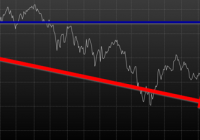
By Wesley R. Gray, Ph.D. Chasing the Investing Unicorn: Give me “High Returns with Limited Risk” Having your cake and eating it too is a great way to go. It’s great to have the cake, and it’s also great to eat the cake. But you can’t have it both ways. This trend continues when we speak with fellow investors: “Give me high, after-tax, net of fee returns, but with limited risk and volatility.” Now, we certainly love high returns with low risk. We also love high reward with low effort and high calories with low weight gain. Unfortunately, this brings us to our first problem with the investing unicorn: Problem #1: Unicorns don’t exist, and neither do high returns with low risk. Unless you are my youngest daughter, age 3, unicorns don’t exist. Sadly, high-return assets with low-risk profiles don’t exist either. Assets that earn high returns, such as equities (e.g., an S&P 500 index fund), come with a lot of risk (i.e., you can lose over half your wealth). The only way to earn high returns, but limit the risk, is to develop a timing methodology that identifies how to sell the high-returning asset before it decides to jump off a fiscal cliff. Which brings me to another kink in the high-reward, low-risk paradox: Problem #2: Market-timing is extremely difficult. Let’s start this conversation with a concise summary of a 55-page academic analysis of a variety of systems that claim to have perfect market-timing ability: Trying to perfectly time the market is a waste of time. There you go. You no longer need to read this classic academic paper in which Ivo Welch and Amit Goyal assess market timing variables. Our own research over several years confirms this sad reality. We’ve reviewed hundreds of different concepts, and the results are not promising. Most signals never “survive” intense empirical scrutiny, and we are generally skeptical of ANY system that purports to work all the time. Simply stated: Nothing works ALL the time . If unicorns don’t exist (high returns, low risk), is there any good news? There is a glimmer of light at the end of this investing tunnel. Specifically, academic research indicates that investors who can stomach short-term volatility, avoid benchmark comparison, and follow a model can systematically outperform over long periods of time. We find the same conclusion with what we call “downside protection.” Historically, two elements provide downside protection: Focus on Strong Absolute Performance Focus on Strong Trending Performance Of course, past performance is certainly no guarantee of future performance ; nonetheless, historically, these methodologies have worked. They haven’t eliminated short-term volatility, and one can be sure they will underperform a buy-and-hold index at some point; however, they have protected portfolios from the most extreme loss situations. Let’s explore a simple downside protection tool and what the evidence to-date can show us. Rule 1: If weak absolute performance appears, go to cash. In the illustration below, the white line represents an asset class with poor absolute performance. In general, avoid assets with poor absolute performance. (click to enlarge) For illustration purposes only. Rule 2: If weak trending performance appears, go to cash. In the illustration below, the purple line represents a long-term trend line (e.g., a moving average) and the white series represents real-time prices. The red circle highlights a point where the real-time price falls below the long-term average. In general, avoid assets with poor trending performance. For illustration purposes only. Do these simple tools work? Let’s look at the data. Moskowitz, Ooi, and Pedersen, in a formal academic paper, highlight that technical rules don’t work all the time, but they have been effective at providing downside protection, historically: “We document significant ” time series momentum ” in equity index, currency, commodity, and bond futures for each of the 58 liquid instruments we consider… … A diversified portfolio of time series momentum strategies across all asset classes delivers substantial abnormal returns with little exposure to standard asset pricing factors and performs best during extreme markets.” – Moskowitz, Ooi, and Pedersen (2012) While market timing systems that work 100% of the time are impossible, we see that some systems, if followed over long periods, can work over time. It all gets back to model discipline and exploiting the behavioral biases of the market (something we love). Let’s simplify the complex analysis presented in formal academic research and focus on replicating these 2 simple rules. Let’s call our system, the “Downside Protection Model”: The Downside Protection Model ((NYSE: DPM )) follows two simple rules: Time Series Momentum Rules (TMOM) Simple Moving Average Rules (MA) Let’s review the details of our simple rules: Absolute Performance Rule: Time Series Momentum Rule (TMOM) Excess return = Total return over past 12 months less return of T-Bills If Excess return > 0, go long risky assets. Otherwise, go long alternative assets (T-Bills) Trending Performance Rule: Simple Moving Average Rule (MA) Moving Average (12) = Average 12-month prices If Current Price – Moving Average (12) > 0, go long risky assets. Otherwise, go long alternative assets (T-Bills). We need a way to combine these two principles in a simple way. We find that complexity does not add value , and simple models beat experts. We extend this belief to downside protection by keeping it simple: We create a Downside Protection Model (DPM) rule, which is 50 percent Absolute Performance (TMOM) and 50 percent Trending Performance (MA): DPM Rule: 50% TMOM, 50% MA Below is a figure that illustrates the basic trading rules we apply to provide downside protection on portfolios: (click to enlarge) The rule is simple: Trigger one rule = go to 50% cash. Trigger both rules = go to 100% cash. No rules triggered = go long. How has the Downside Protection Model performed? We provide a series of tests on the Downside Protection Model, applied to generic market indices. Our core samples includes 5 asset classes, assessed over the 1973-2014 time period: SPX = S&P 500 Total Return Index EAFE = MSCI EAFE Total Return Index LTR = The Merrill Lynch 10-year U.S. Treasury Futures Total Return Index REIT = FTSE NAREIT All Equity REITS Total Return Index GSCI = S&P GSCI Total Return CME Results are gross, no fees are included. All returns are total returns and include the reinvestment of distributions (e.g., dividends). Data sources include Bloomberg. Indexes are unmanaged, do not reflect management or trading fees, and one cannot invest directly in an index. Comparison #1: Looking at these basic rules individually: Absolute Performance (TMOM) vs. Trending Performance (MA) Before we compare the system as a whole, let’s compare each rule against the other to see if one is particularly more effective. From January 1, 1976 through December 31st, 2014, here is what we find: TMOM wins 60% of the time, MA wins 40% of the time (Win = better Sharpe and Sortino; Loss = Sharpe and Sortino worse; Tie = a combination of some sort) TMOM triggers around 20% less than MA does (number of triggers refers to the number of times the rule breaks out of the asset class and goes to T-Bills) Bottom Line: Both rules have been effective at providing downside protection. Below are the stats. (click to enlarge) The results are hypothetical, are NOT an indicator of future results, and do NOT represent returns that any investor actually attained. Indexes are unmanaged, do not reflect management or trading fees, and one cannot invest directly in an index. Additional information regarding the construction of these results is available upon request. Comparison #2: Assess the Downside Protection Model (DPM): Absolute Performance (TMOM) plus Trending Performance (MA) Now, let’s combine the rules into our simple Downside Protection Model ( DPM ) and see if any incremental improvement occurs. Here is what we find: Downside Protection Model (DPM) wins overall (Win = better Sharpe and Sortino; Loss = Sharpe and Sortino worse; Tie = combination of some sort). Bottom Line: Combining the rules into a single Downside Protection Model (DPM) appears to work. (click to enlarge) The results are hypothetical, are NOT an indicator of future results, and do NOT represent returns that any investor actually attained. Indexes are unmanaged, do not reflect management or trading fees, and one cannot invest directly in an index. Additional information regarding the construction of these results is available upon request. Note: Additional robustness tests are available in the appendix. Are these results sustainable? The basic results above highlight that DPM significantly reduces the realized maximum drawdown on a portfolio. But perhaps the entire exercise above is an example of data mining and over-optimization. Nobody can ever prove, beyond any doubt, that a Downside Protection Model works. There is always a chance that any historical finding is driven by randomness, and thus, past performance will not reflect future performance. In the Appendix section below, we stress test this system across numerous time periods and different markets, all of which present similar conclusions. However, we believe there is a behavioral story underlying the success of our simple downside protection rules. Consider the concept of dynamic risk aversion, which is the idea that human beings don’t stick to a set risk/reward behavior – their appetite for risk can change depending on their recent experience. For example, imagine we are making a decision to build a new house in California along the San Andreas Fault. If we just lived through an earthquake, taking on the risk of building a new house on the San Andreas Fault is probably scarier, even though the probability of another earthquake may not have changed. In contrast, when there hasn’t been an earthquake in fifty years, building a new house along a fault is not a big deal. As this example shows, our perception of risk is not constant, and can change based upon recent experience (if you doubt this example, kindly look at a picture of San Francisco’s skyline). In terms of market crashes, we will likely overreact to extreme times and underreact to peaceful times, despite the statistical probability to the contrary. Another assumption economists sometimes make is that risk, often measured in terms of standard deviation, or “volatility,” is relatively constant. These assumptions are challenged when extreme stock market drawdowns occur. Let’s look at another example: a 50% market correction, when fundamentals imply a 20% correction is sufficient. As market prices drop below the twenty percent threshold, an economist assumes that the new price is a bargain. Expected returns have gone up after prices have moved down, while volatility and risk aversion are assumed to be relatively constant. Implicitly, investors should swoop in to buy these cheap shares and bring the market to equilibrium (which, in our example, is their so-called fundamental value). But this doesn’t happen. Stocks can – and have – gone down over fifty percent, and these movements are much more volatile than the underlying dividends and cash flows of the stocks they represent! Remember 2008/2009? How many investors swooped in to buy value versus threw the baby out with the bathwater and kept selling? One approach to understanding this puzzle is by challenging the assumption that investors maintain a constant aversion to risk. Consider the possibility that investors change their view on risk after a steep drawdown (i.e., they just lived through an earthquake). Even though expected returns go up dramatically, risk aversion shoots up dramatically as well. This change means prices have to go down a lot further to justify an investment in these “cheap” stocks. This heightened aversion to risk – following a steep price drop – leads to more selling, and more selling leads to even more hate for risk, which leads to more selling, and so forth. What you end up with is a stampede for the exit and an intense sell-off in the marketplace – below fundamental value, and well beyond what a traditional economist would consider “rational.” The discussion above is a simplified story of investor psychology in the context of a stock market drawdown. For exposition purposes, we are leaving out many potentially important details. However, if one believes that investors rethink their tolerance for risk during a market debacle and tend to sell shares at any price, this might help explain why long-term trend-following rules, which systematically get an investor out of a cliff-diving bear market before everyone has jumped ship, have worked over time. Of course, technical rules will only work if the massive bear market doesn’t happen in a short time period before the long-term trend rules can signal an exit. Technical rules will not save an investor from a 1987-type “flash” crash, but they can save an investor from a 1929- or a 2008-type crash, which can take a few months to develop. In the end, if one believes in a price dynamic that involves steep and relatively sharp declines, followed by slow grinding uphill climbs, simple technical rules will, by design, improve risk-adjusted performance. Conclusion Simple timing rules, focused on absolute and trending asset class performance, seem to be useful in a downside protection context. Our analysis of the downside protection model (DPM), applied on various market indices, indicates there is a possibility of lowering maximum drawdown risk, while also offering a chance to participate in the upside associated with a given asset class. Important to note, applying the DPM to a portfolio will not eliminate volatility, and the portfolio will deviate (perhaps wildly) from standard benchmarks. For many investors, these are risky propositions and should be considered when using a DPM construct. Note: We will be implementing a version of our downside protection model with our new automated advisor offering, Alpha Architect Advisor . Appendix Robustness test of the DPM model across time periods and markets Subperiod: 01/01/1976-12/31/1995 DPM is 50% invested in a TMOM strategy and 50% invested in an MA strategy. Strategies invest in T-bills when a trading rule triggers. DPM wins 3/5, B&H wins 1/5, DPM ~ B&H 1/5 (Win = Sharpe & Sortino; Loss = Sharpe & Sortino; Tie = other) Bottomline: TMOM and MA provide downside protection. (click to enlarge) The results are hypothetical, are NOT an indicator of future results, and do NOT represent returns that any investor actually attained. Indexes are unmanaged, do not reflect management or trading fees, and one cannot invest directly in an index. Additional information regarding the construction of these results is available upon request. Subperiod: 01/01/1996-12/31/2014 Bottom Line: DPM holds and provides better protection. (click to enlarge) The results are hypothetical, are NOT an indicator of future results, and do NOT represent returns that any investor actually attained. Indexes are unmanaged, do not reflect management or trading fees, and one cannot invest directly in an index. Additional information regarding the construction of these results is available upon request. Out of Sample Test #1-> U.S. Market (01/01/1928-12/31/1975) Our core sample includes 1 asset class, assessed over the 1928-1975 time period: SPX = S&P 500 Total Return Index Results are gross, no fees are included. All returns are total returns and include the reinvestment of distributions (e.g., dividends). Data sources include Bloomberg. Indexes are unmanaged, do not reflect management or trading fees, and one cannot invest directly in an index. Both TMOM and MA work well for downside protection, significantly lowering total drawdowns. Strategies invest in T-bills when a trading rule triggers. Bottomline: TMOM and MA provide downside protection and have similar results to the Downside Protection Model. (click to enlarge) The results are hypothetical, are NOT an indicator of future results, and do NOT represent returns that any investor actually attained. Indexes are unmanaged, do not reflect management or trading fees, and one cannot invest directly in an index. Additional information regarding the construction of these results is available upon request. Drawdown Comparison Both TMOM and MA significantly lower downside risk when the top drawdowns of the buy-and-hold benchmark occurs. MA and TMOM provide similar drawdown protection during buy-and-hold drawdowns. TMOM and MA protect capital at different times (see bold text below). Bottomline: Downside Protection Model diversifies risk management by combining the rules. (click to enlarge) The results are hypothetical, are NOT an indicator of future results, and do NOT represent returns that any investor actually attained. Indexes are unmanaged, do not reflect management or trading fees, and one cannot invest directly in an index. Additional information regarding the construction of these results is available upon request. Out of Sample Test #2 -> Japanese and German Stock Markets Our robustness samples include 2 global markets (Japan and Germany): NKY = Nikkei 225 Index (1971 to 2014) DAX = Deutsche Boerse AG German Stock Index (1961 to 2014) Results are gross, no fees are included. All returns are price returns and DO NOT include the reinvestment of distributions (e.g., dividends). Data sources include Bloomberg. Indexes are unmanaged, do not reflect management or trading fees, and one cannot invest directly in an index. We use zero as the alternative asset return when a trading rule is triggered. Nikkei Summary Results (1971-2014): Both TMOM and MA work well on drawdown protection. TMOM works slightly better overall. TMOM has the highest return during this period. DPM lowers the sum of total drawdowns by a material amount. NKY_DPM (TMOM and MA): Equal weight on NKY_TMOM and NKY_MA; portfolio earns zero returns when flat. NKY_TMOM: Times series momentum applied on NKY with 12-month formation window, and earns zero returns when flat. NKY_MA: 1-month and 12-month MA rule applied on NKY and earns zero returns when flat. NKY_B&H: Buy and hold on Nikkei 225 price-only series. (click to enlarge) The results are hypothetical, are NOT an indicator of future results, and do NOT represent returns that any investor actually attained. Indexes are unmanaged, do not reflect management or trading fees, and one cannot invest directly in an index. Additional information regarding the construction of these results is available upon request. Drawdown Comparison (Nikkei) Both TMOM and MA significantly lower downside risk during the top drawdowns of the buy-and-hold benchmark. MA and TMOM provide similar drawdown protection during buy-and-hold drawdowns. TMOM and MA protect capital at different times (see bold). The Downside Protection Model is diversifying risk management. (click to enlarge) The results are hypothetical, are NOT an indicator of future results, and do NOT represent returns that any investor actually attained. Indexes are unmanaged, do not reflect management or trading fees, and one cannot invest directly in an index. Additional information regarding the construction of these results is available upon request. DAX Summary Results (1961-2014) Both TMOM and MA work well on drawdown protection. TMOM has higher CAGR and lower drawdown. The Downside Protection Model is roughly equivalent to TMOM with lower Max Drawdown. DAX_50,50 (TMOM and MA): Equal weight on DAX_TMOM and DAX_MA; portfolio earns zero returns when flat. DAX_TMOM: Times series momentum applied on DAX with 12-month formation window and earns zero returns when flat. DAX_MA: 1-month and 12 month MA rule applied on DAX and earns zero returns when flat. DAX_B&H: Buy and hold on DAX 40 price-only series. (click to enlarge) The results are hypothetical, are NOT an indicator of future results, and do NOT represent returns that any investor actually attained. Indexes are unmanaged, do not reflect management or trading fees, and one cannot invest directly in an index. Additional information regarding the construction of these results is available upon request. Drawdown Comparison (NASDAQ: DAX ) Both TMOM and MA significantly lower downside risk during the top drawdowns of the buy-and-hold benchmark. MA and TMOM provide similar drawdown protection during buy-and-hold drawdowns. TMOM and MA protect capital at different times (see bold). The Downside Protection Model is diversifying risk management. (click to enlarge) The results are hypothetical, are NOT an indicator of future results, and do NOT represent returns that any investor actually attained. Indexes are unmanaged, do not reflect management or trading fees, and one cannot invest directly in an index. Additional information regarding the construction of these results is available upon request. Statistics Definitions CAGR: Compound Annual Growth Rate Standard Deviation: Sample standard deviation Downside Deviation: Sample standard deviation, but only monthly observations below 41.67 bps (5%/12) are included in the calculation. Sharpe Ratio (annualized): Average monthly return minus Treasury bills divided by standard deviation Sortino Ratio (annualized): Average monthly return minus Treasury bills divided by downside deviation Worst Drawdown: Worst peak-to-trough performance (measured based on monthly returns) Mathematical Relationship Between TMOM and MA (click to enlarge) The results are hypothetical, are NOT an indicator of future results, and do NOT represent returns that any investor actually attained. Indexes are unmanaged, do not reflect management or trading fees, and one cannot invest directly in an index. Additional information regarding the construction of these results is available upon request. Original Post